Attention mechanism in conditional models.
Some used references (more throughout the text)
[1] UvA deep learning course transformers and vision transformers
[2] Lilian Weng attention blogpost
Motivation
I have been working in gene regulation, particularly in condition-specific gene regulation. This boils down to combinatorics of motifs, protein-protein and protein-dna interactions (see this). Deep learning might be a good framework to study this phenomena. On the first steps I want to ignore the specifics of protein representations and just try to see how the motifs or segments of DNA that are relevant to expression change for different conditions.
So far, I have been using a very primitive network (see publication here). However, this relies on a MLP to model the interactions of motifs and treatment embeddings. The modern take on conditional neural networks is surely transformers. What the network focuses on depends on the context, in general, of the input itself, through self-attention. My idea here is to use (cross-)attention (not self-attention) between some treatment embedding and dna embedding. In that way, I aim to construct a model that focuses in different areas of the promoter region for different treatments, furthermore, attention matrices might be interpretable. Here I aim to get an overview of how attention mechanism are used to combine different data sources or condition the network to some extra input.
Introduction:
The seminar work on attention is Neural Machine Translation By Jointly Learning To Align and Translate:
“The most important distinguishing feature of this approach from the basic encoder–decoder is that it does not attempt to encode a whole input sentence into a single fixed-length vector. Instead, it encodes the input sentence into a sequence of vectors and chooses a subset of these vectors adaptively while decoding the translation.”
Essentially, in this work they compute a context vector as a weighted sum of the hidden states of a RNN (this is running over a sequence of words/tokens). The weights are calculated using some function (they use an MLP) of the similarity between the hidden state of the decoder at time t and the hidden states of the encoder over the whole sequence and then using softmax.
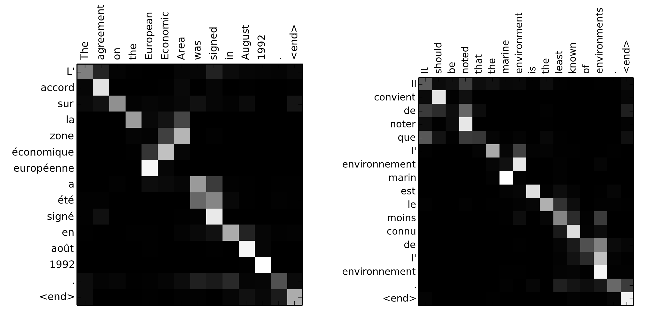
\[\alpha_{i, j} = \frac{\exp{e_{ik}}}{\sum_{k=1}^T\exp(e_{ik})}\]Where \(e_{ik}\) is some similarity score between the two hidden states (from encoder and from decoder). In essence, this normalized similarity can be understood as the probability that the target word \(y_i\) is aligned to, or translated from, a source word \(x_j\). In a typical RNN the hidden state of the encoder would depend on words up to \(j\). However, they propose a bidirectional RNN. They want that the hidden state takes into account the whole context above and below.
These normalized similarities can be framed into an adjacency matrix (not necessarily squared!), such as below (from the same paper):
Text-Image interaction, RNNs and attention
The following approaches are interesting because of the interpretability side effects (note that DNA may be framed as a 1D image…), see the following image:
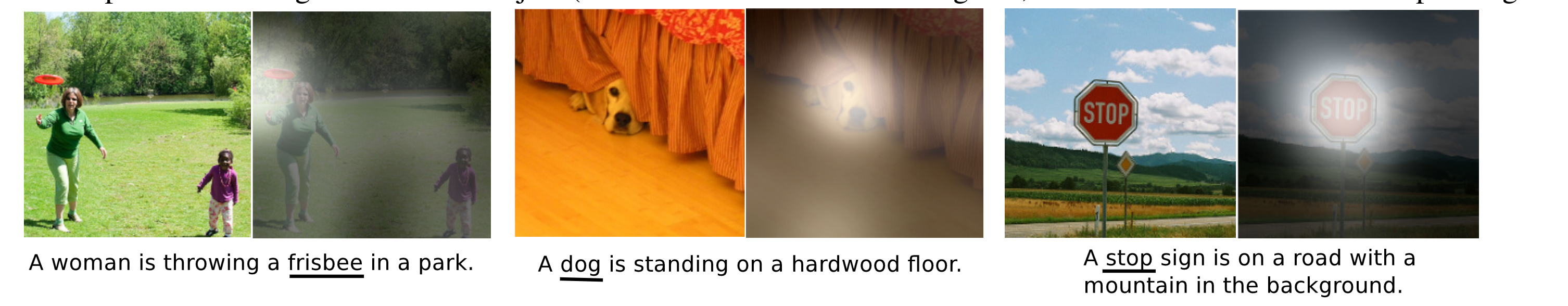
The above image comes from: Show, Attend and Tell: Neural Image Caption Generation with Visual Attention where they use attention on embeddings of an image derived from a CNN. This allowed them to compute where in the image the attention was focused on (this is a very interesting feature for dna-protein interaction prediction). Particularly, they aim to label images, and could relate hidden state \(\mathbf{h}_{t-1}\) to a particular embedding and hence to an area in the image. For
\[\{\mathbf{a_1}, ..., \mathbf{a_L}\}\]being the embeddings of a particular position (on a lower resolution representation of the image due to pooling layers), output of the last layer of a CNN. Hence each of those vectors has dimensionality equal to the number of feature maps. They construct a function that selects a particular position vector representation (or a computes a weighted sum) to predict the next word. To interpret which part of the image the network was attending to, they upscale the selected positional vector (or attention distribution over the positional vectors) to the original resolution using some smoothing function.
The attention is calculated with an “attention model” and a softmax function. They define \(f_{att}\) using a MLP. This network takes the hidden state of the LSTM and a position vector and outputs an activation that is then passed through a softmax function to calculate the attention weight \(\in (0, 1)\):
\[\alpha_{ti} = \frac{\exp(f_{att}(\mathbf{a_i},\mathbf{h}_{t-1}))}{\sum_{k=1}^{L} \exp(f_{att}(\mathbf{a_k},\mathbf{h}_{t-1}))}\]It is also relevant to notice that here there is only one attentional layer. So the network attends only to a particular location at each time. This is in contrast to modern multi-head attention approaches, as I describe below.
Stacked Attention Networks for Image Question Answering focuses on answering questions related to an image. A CNN is used to extract high level image representations, same as before. Again, they focus on the position vector representation. For instance, if the last layer outputs 14x14x512 (height, width, channels), there are \(14^2\) different vectors of length 512. Indeed, these are related to a particular area of the image, depending on the receptive field of the network.
Then, they also use a question model, an LSTM on the text. Given the image feature matrix \(\mathbf{V}_I\) (as per they definition, this is a matrix with 14x14 columns and 512 rows) and the question feature vector \(\mathbf{V}_Q\) they calculate a softmax score per each region in the image using a single layer neural network with hyperbolic tangent activation and then softmax. This yields the attention probability of each image region given the question. With that, they get a weighted average of the image (over the different positions), getting a vector of length 512. Since their text embedding has the same dimensionality they add those up to form an enriched query. Importantly, in this work they already implement several attention layers one after another (not in parallel).
Again, in order to visualize the attention, they upscale the 14x14 distribution to the original resolution 448x448 using a Gaussian filter.
Transformers
In Attention is all you need they remove any convolutions or RNNs from the architecture. They use self-attention to compute encoder and decoder hidden states (instead of an RNN, such as a bidirectional RNN) and they use attention to map hidden states of encoder and decoder (the latter, same as before).
The key points of this architecture are its speed (no need for recurrence, no need for convolutions) and its easy parallelism. Parallelism is easy because the hidden representation can be separated in several vectors and attention can be calculated for each of these. This parallelism does not yield a computational advantage but a flexibility one. Now similarities, are computed over several representations instead of just one. This allows for more diversity of interactions between hidden representations.
Being this such a crucial architecture it is important to dive into details:
Let \(\mathbf{Q} \in \mathbb{R}^{T \times d_k}\), \(\mathbf{K} \in \mathbb{R}^{T \times d_k}\) and \(\mathbf{V} \in \mathbb{R}^{T \times d_v}\). Then
\[\mathbf{e} = \frac{QK^{\top}}{\sqrt{d_k}} \in \mathbb{R}^{T\times T}\]Dividing by the square root of the embedding dimension here is important to counteract the effect of the length of the embedding dimension in the magnitude of the dot products.
Then, normalize each row in \(\mathbf{e}\) using softmax, let us call it \(\mathbf{A} \in (0, 1)^{T \times T}\). Note that this the same as above, the difference is that in the definitions above the attention is defined just for one element (hence yielding a vector and not a matrix). In the definitions above \(\alpha\) had usually two subscripts, but one was kept fix.
The “Scaled Dot-Product Attention”:
\[\text{Attention}(\mathbf{Q, K, V}) = \text{Softmax}\left(\frac{\mathbf{QK}^{\top}}{\sqrt{d_k}}\right)\mathbf{V} = \mathbf{A}\mathbf{V} \in \mathbb{R}^{T \times d_v}\]The “\(\text{Softmax}\)” notation is indeed very confusing. Note that the first dimension of \(\mathbf{Q}\) and \(\mathbf{K}\) do not need to be equal. The requirement is that the first dimension in \(\mathbf{K}\) and \(\mathbf{V}\) be equal (which means that Key and Value must always be the same). So indeed \(\mathbf{A}\) could be a rectangular matrix. And in fact, in the transformer, in the “encoder-decoder” attention layers, there should be no requirement for \(\mathbf{A}\) to be square, since it could be dealing with different languages (hence a sentence could be of different length).
This last point (which is clear on the previous approaches) is not so clear here, but is very important for using attention-like architectures for conditional models. When the embeddings come from different sequences they call it “cross-attention”” instead of “self-attention”. Indeed, “Cross-attention” is simply the attention architecture when it is not applied to itself, i.e. “mixes” two different embedding sequences (this is exactly what I am looking for).
Now, making it in parallel:
Essentially, the idea is to truncate the embedding dimension into \(h\) elements of size \(d_k\). In that way, several parallel attention matrices \(\mathbf{A}\) can be computed. This is advantageous because you may want to attend to different elements of a sequence.
Importantly, here they include learnable parameters (and there should be learnable parameters even if parallelism is not applied, otherwise the dot product is limited to some “given” representation). For each head \(h\), there will be matrices for query and key \(\mathbf{W}^Q, \mathbf{W}^Q \in \mathbb{R}^{D \times d_k}\), for value \(\mathbf{W}^V \in \mathbb{R}^{D \times d_v}\) and a matrix for the concatenated output \(\mathbf{W}^O \in \mathbb{R}^{h\cdot d_v \times d_out}\)
As a final note, the position of the elements in the sequence is lost. Transformers treat them as elements of a set. In the original transformer paper they use a 50 dimensional positional encoding based on trigonometric functions with different frequencies.
transformers, graphs and pruning heads
This blogpost gives a very intuitive explanation on why attention layers are a form of message passing algorithm. They compute a weighted aggregation of representations based on learned similarities. This is why attention matrices can be insightful (even more so in scientific applications). However, having several heads makes it more difficult to extract insight (note that first uses of attention did not use several heads).
Here they propose an algorithm for pruning heads, and also show that this can be done without drastic performance changes. They note that encoder-decoder attention layers are much more reliant on multi-head than the self-attention layers.
Conditional diffusion
In a previous post I studied diffusion models (from the perspective of score matching) as a way to approximating the gradient of a data distribution. In that post, however, I did not dive into conditional gradients. This is, I focused on sampling from \(p(\mathbf{x})\) and not sampling from a conditional distribution \(p(\mathbf{x}|y)\). In image generation this conditional distribution is key, and this condition is what is known as the prompt in text-to-image models.
Now, what I am interested here is how the gradient is conditioned with the prompt. Following this lets first dive into classifier guidance:
\[\nabla_{\mathbf{x}} \log p(\mathbf{x}|y) = \nabla_{\mathbf{x}} \log \left( \frac{p(\mathbf{x})p(y|\mathbf{x})}{p(y)} \right) = \nabla_{\mathbf{x}} \log p(\mathbf{x}) + \nabla_{\mathbf{x}} \log p(y|\mathbf{x})\]The first term is basically the diffusion model and the second term is the gradient of a classifier, this is, the change in the probability of class \(y\) with respect to the elements in \(\mathbf{x}\). Hence, you can stir the sampling direction of the diffusion model with the gradient of the classifier. It does, however, require a pre-trained classifier here that is reliable enough with noisy samples.
In Diffusion Models Beat GANs on Image Synthesis they add time-step (of the diffusion process) and class in the normalization layers using “adaptative group normalization (AdaGN)”;
\[\text{AdaGN}(h, y) = y_s \text{GroupNorm}(h) + y_b.\]Where \(h\) are the activations of network and \(y_s, y_b\) are embeddings of time and class (this is also an interesting approach for conditioning a model actually, without attention). However, their main guidance is still a classifier.
Classifier-Free guidance consist on training a conditional and unconditional model simultaneously, essentially it uses the class as input to the network or a ‘None’ class for the unconditional one.
In the Stable Diffusion paper they turn their diffusion model into a more flexible conditional image generator by augmenting the UNet backbone with “cross-attention”. Indeed, as I mentioned above, the attention mechanism in the Transformer must have “cross-attention” at the connection between encoder and decoder. And in general, previous RNN/CNN based encoders with attention only used “cross-attention” (so indeed, “cross-attention” is the general case). They create a domain specific encoder \(\tau_{\theta}\) that generates an embedding of the prompt \(\tau_{\theta}(y) \in \mathbb{R}^{M \times d_{\tau}}\). This is mapped to intermediate layers of the UNet through attention. Where \(\mathbf{Q} = \mathbf{W}^{i}_Q \cdot \phi_i(\mathbf{x}), \mathbf{K} = \mathbf{W}^{i}_k \cdot \tau(y), \mathbf{V} = \mathbf{W}^{i}_V \cdot \tau(y)\), being \(\phi_i(\mathbf{x})\) the flattened intermediate representation in the UNet. Being the the matrices \(\mathbf{W}\)s learnable projection matrices. Since there are plenty of residual connections in the UNet it is not problematic that the attention values are the text embeddings, since the image material will be passed through the network as well. In that sense, the attention output relates a particular token with some locations in the image. Particularly, the output of the attention is the weighted combination of the token embeddings for different locations in the image.
Note that the UNet is the backbone of this algorithm, and it is used in every step of the generation! The encoder \(\tau_{\theta}\) (they use a transformer here) must be trained simultaneously with whole UNet.
Vision transformers
Applying transformers to images seems counterintuitive (given the magnificent inductive biases that CNN have). And indeed they require a patching pre-processing step. The patches then are considered as elements of a sequence. This does not seem to be particularly relevant for me here beyond the fact that they indeed need to do patches, so attention on top of convolution features is indeed not a “weird thing”.
Take away message:
What are the options to do conditional classification of promoter sequence? Possibly the bests calls for a “modern” architecture are some CNN + multihead cross-attention with treatment embeddings. Which is the simple and most interpretable option. Or, a much more cumbersome conditioning throughout the network, such as the one in the stable diffusion paper. Exchanging the CNN by a pre-trained transformer might also be an option, even more cumbersome, however (I am also not so sure that those are that superior to CNNs…).
Now is time to dive into the details of CNN architectures in DNA modelling…