Optimal Separating Hyperplanes
References:
The following notes are mostly based on the following sources:
[1] Elements of Statistical Learning
[2] Numerical optimization, Nocedal
[3] Khan Academy (Lagrange multipliers, by 3blue1brown)
[4] Lagrangian Duality for Dummies
Introduction
Now that everyone is looking into Large Language Models (me included) I wanted to get back to the basics, to the more mathematically precise. For a while, I wanted to implement Support Vector Machines (SVMs) from scratch and this podcast motivated me to do it. Eventually, I want to get into the invariances that Vladimir Vapnik talks about, which, as I see it, quite resemble the ideas in geometric deep learning.
In any case, SVMs are not trivial, when I went through them in class (just one lecture!) I did not get anything, and Elements Of Statistical Learning is not very explicit. So, in this post I start with the optimal separating hyperplanes problem, focusing on the geometry. I let the SVMs for a second post.
So, we are looking for a hyperplane that optimally separates data into two classes. We aim to find the hyperplane that maximizes the margin between the two classes. This works only when the data are linearly separable. However, we can always expand the basis where our data lives to be able to separate it, at the cost of possibly overfitting.
Geometrical details.
First, let’s define the separating hyperplane:
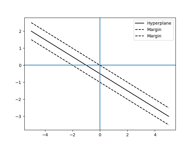
\[\mathbf{\beta}^T\mathbf{x} + \beta_0 = 0\]We are interested in the set: \(H = \{\mathbf{x} \in \mathbb{R}^n : \mathbf{\beta}^T\mathbf{x} + \beta_0 = 0\}\). Note that \(\mathbf{\beta}\) is a vector of n dimensions and \(\beta_0\) a scalar. These points are equidistant from the two hyperplanes \(S1 = \{\mathbf{x} \in \mathbb{R}^n : \mathbf{\beta}^T\mathbf{x} + \beta_0 = 1\}\) and \(S2 = \{\mathbf{x} \in \mathbb{R}^n : \mathbf{\beta}^T\mathbf{x} + \beta_0 = -1\}\). Those hyperplanes will pass through the support vectors (more on this later).
This is very similar to logistic regression. In logistic regression, we construct a function \(\mathbb{R}^n \rightarrow [0, 1]\) and then we classify points based on whether they are above or below some probability threshold (e.g. 0.5). Indeed, by fixing a threshold we define a hyperplane. In SVMs, we construct a function \(\mathbb{R}^n \rightarrow \mathbb{R}\) and then we classify points based on whether they are above 1 or below -1. However, we expect SVMs to generalize better since the margin in this classification is maximized.
To plot this say for \(\mathbf{x} \in \mathbb{R}^2\), \(\mathbf{\beta} = [1, 2]\) and \(\beta_0 = 1\) we just need to realize that \(\mathbf{\beta}^T\mathbf{x} + \beta_0 = 0\) is the same as \(b_0 x_1 + b_1 x_2 + \beta_0 = 0\). So given \(x_1\) we can find \(x_2\) and vice versa:
\[x_2 = \frac{-\beta_0 - b_0 x_1}{b_1}\]The same idea applies to higher dimensions.
Now, we want to find \(\mathbf{\beta}\) and \(\beta_0\) that maximize the margin between the two hyperplanes so first we need to define this distance. To do so we use the normal (perpendicular vector, often of unit length) to the hyperplanes.
To find the normal to a hyperplane we first define a vector parallel to the hyperplane; any vector that goes from one point to another in the hyperplane. We can accomplish this by setting the starting point of \(\mathbf{x}_1\) to \(\mathbf{x}_2\) such that \(\mathbf{v} = \mathbf{x}_1 - \mathbf{x}_2\). What is important, however, is the direction, which is given by \(\mathbf{v}\). The normal \(\mathbf{w}\) to the hyperplane must be such that \(\mathbf{w}(\mathbf{x}_1 - \mathbf{x}_2)=0 \quad \forall \quad \mathbf{x}_1, \mathbf{x}_2 \in H\). This \(\mathbf{w}\) is given by \(\frac{\mathbf{\beta}}{\lVert\beta\rVert}\) (dividing by the norm to get unit length) by the definition of the hyperplane \(H\).
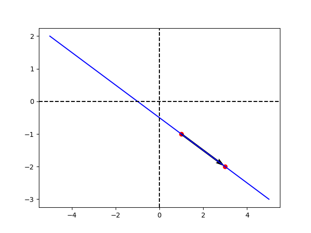
To find the distance between two hyperplanes, S1 and S2, we focus on a given point \(\mathbf{x}_1 \in S1\). Let’s find the point in S2 in the direction of the perpendicular from \(\mathbf{x}_1\). The perpendicular line that passes through \(\mathbf{x}_1\) is given by \(\mathbf{x}_1 + m\frac{\mathbf{\beta}}{\lVert\beta\rVert}\). For \(m\) being… the margin!
Again, divide \(\mathbf{\beta}\) by its norm to get a unit vector there. Clearly, for m = 0, it intersects \(\mathbf{x}_1\). Which is the corresponding x in S2?
We know that \(\mathbf{\beta}^T(x_1 + m\frac{\mathbf{\beta}}{\lVert\beta\rVert}) + \beta_0 = -1\) for some \(m\), which is precisely the number we want to find. So with some algebra;
\[\mathbf{\beta}^T x_1 + m\frac{\lVert\beta\rVert^2}{\lVert\beta\rVert} + \beta_0 = -1\] \[\mathbf{\beta}^T x_1 + m\lVert\beta\rVert + \beta_0 = -1\] \[m = \frac{-\mathbf{\beta}^T x_1 - \beta_0 - 1}{\lVert\beta\rVert}\]And from the definition of S1, we know \(\beta^T x_1 = 1 - \beta_0\),
\[m = \frac{-1 + \beta_0 - \beta_0 - 1}{\lVert\beta\rVert} = \frac{-2}{\lVert\beta\rVert} \propto \frac{1}{2}\frac{1}{\lVert\beta\rVert}\]And that is the definition of the margin, it is inversely proportional to the norm of \(\beta\). Importantly, we only care about its absolute value. It is relevant to notice that this function will be maximized at the same point as \(\frac{1}{\lVert\beta\rVert^2}\), this is important because it will make the optimization problem easier.
To me, that result was not intuitive, let’s see this in action:
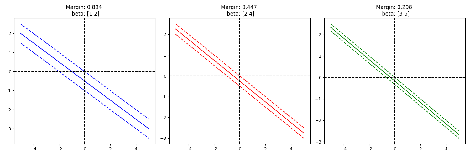
Yep, it seems to work… Intuitively, given a direction, we can think of the increase/decrease in \(\mathbf{\lVert x \rVert}\) that is required to move from one hyperplane to the other (e.g. from S1 to S2). The bigger the sensitivity to \(\mathbf{x}\) the less we need to move to get a change of hyperplane. This is why minimizing the norm of \(\mathbf{\beta}\) is equivalent to maximizing the margin.
Optimal Separating Hyperplane problem formulation.
Now we have the geometrical background to frame the problem:
We can do this by minimizing \(\frac{1}{2}\lVert\beta\rVert^2\). However, we need to make sure that this hyperplane separates the data correctly. We can do this by subjecting this minimization process to the constraint of \(y_i(\mathbf{\beta}^T\mathbf{x}_i + \beta_0) \geq 1 \quad \forall \quad i = 1, \dots, n\). Being \(y_i\) the class of \(\mathbf{x}_i\) which is eihter 1 or -1. This constraint is equivalent to saying that the point is on the right side of the hyperplane and with enough margin. Negative values imply wrong classification, values between 0 and 1 imply that the point is between the two hyperplanes, which is not what we want. Finally, the problem is:
\[\min_{\mathbf{\beta}, \beta_0} \frac{1}{2}\lVert\beta\rVert^2\] \[\text{s.t.} \quad y_i(\mathbf{\beta}^T\mathbf{x}_i + \beta_0) \geq 1 \quad \forall \quad i = 1, \dots, n\]This is the same formulation given in Elements of Statistical Learning (they arrive here in a very confusing way imho). The solution to this problem is far from trivial and requires going rapidly over some optimization theory.
Optimization process.
Constrained optimization (Lagrangian).
The idea of the Lagrangian is based on the fact that the gradient of the function we are optimizing and the gradient of the constraint are proportional at the optimum. The proportionality constant is called the Lagrange multiplier. The Lagrangian is just the way of packing up that information in a way that, when optimizing the Lagrangian w.r.t the original variables and the Lagrange multiplier, we are just finding the proportionality constant and satisfying the constraint. Nevertheless, for inequality constraints, as is the case here, the Lagrangian is not (directly) enough. We need to introduce the idea of the KKT conditions.
KKT conditions.
This is a generalization of the method of Lagrange multipliers (Lagrangian). The Karush-Kuhn-Tucker (KKT) conditions are just first-order necessary conditions for a constrained problem, they follow relatively intuitively. They tell you that the Lagrangian must be at a stationary point and the way this has to happen. Equality constraints must be satisfied, inequality constraints that are not active must have a 0 Lagrange multiplier and therefore the “second” part of the Lagrangian is going to add to 0 (either a restriction is active or the Lagrange multiplier is 0). The KKT conditions come as follows:
\[\nabla f(x^*) + \sum_{i \in A} \lambda_i^* \nabla c_i(x^*) = 0\]This just tells us that the Lagrangian must be equal to 0, this means that the gradient of the objective function and constraint function must be proportional (kind of as before). And now, how this must happen:
\[c_i(x^*) = 0, i \in E\]For E the set of equality constraints.
\[c_i(x^*) \leq 0, i \in I\]For I the set of inequality constraints.
\[\lambda_i^* \geq 0, i \in I\] \[\lambda_i^* c_i(x^*) = 0, i \in I \cup E\]Satisfying this is enough to have a first-order optimality condition. Which should be enough for convex problems. Importantly, the satisfied constraints will have a non-cero Lagrange multiplier. In the case of optimal separating hyperplanes, those will be the points corresponding to the support vectors. As we will see later, \(\beta\) is entirely defined as a weighted combination of the support vectors.
Now the issue is, how do we solve this? We have defined some optimality conditions but this is harder than unconstrained problems, what can we do about this?
In Elements of Statistical Learning, they propose to solve this by first simplifying the problem through the dual form and then using a “standard” constrained optimization algorithm. Let’s see how this dual form helps.
Dual-Primal forms.
The idea here is to approximate an infinite penalty for breaking a constraint by a finite, linear penalty. This is done by introducing a new variable \(\mathbf{\alpha}\), which is the Lagrange multiplier for the inequality constraints. In essence, we would have the original problem if \(\alpha = \infty\), and we have a lower bound when \(\alpha \leq \infty\). We can then write the Lagrangian as:
\[\min_{\mathbf{\beta}, \beta_0} \max_{\mathbf{\alpha}} \frac{1}{2}\lVert\beta\rVert^2 - \sum_{i=1}^n \alpha_i (y_i[\mathbf{\beta}^T\mathbf{x}_i + \beta_0] - 1)\]The sign before the Lagrange multipliers here comes from the fact that if we allow for values equal or bigger than 1, then \(\alpha = 0\), but we have to infinitely penalize values smaller than 1, which are elements either wrong classified or between the two hyperplanes. For some intuition, note that in the latter case, \(y_i[\mathbf{\beta}^T\mathbf{x}_i + \beta_0] - 1\) becomes negative, so big positive values of \(\alpha\) will make the Lagrangian big.
That is hard. But if we reverse the order to:
\[\max_{\mathbf{\alpha}} \min_{\mathbf{\beta}, \beta_0} \frac{1}{2}\lVert\beta\rVert^2 - \sum_{i=1}^n \alpha_i (y_i[\mathbf{\beta}^T\mathbf{x}_i + \beta_0] - 1)\]This is what is known as the dual form, which is much more tractable. Now, this will only be the same in some cases (strong duality). Luckily, this is the case for the optimal separating hyperplane problem (and for SVMs).
We can solve the minimization bit of the problem by taking the gradient w.r.t \(\mathbf{\beta}\) and \(\beta_0\) and setting it to 0 (first-order optimality condition). This will (easily) give us the following:
\[\mathbf{\beta} = \sum_{i=1}^n \alpha_i y_i \mathbf{x}_i\] \[\sum_{i=1}^n \alpha_i y_i = 0\]And then plugging this in:
\[\max_{\mathbf{\alpha}} \sum_{i=1}^n \alpha_i - \frac{1}{2} \sum_{i=1}^n \sum_{k=1}^n \alpha_i \alpha_j y_i y_k \mathbf{x}_i^T \mathbf{x}_k\] \[\text{s.t.} \quad \sum_{i=1}^n \alpha_i y_i = 0 \text{ and } \alpha_i \geq 0 \quad \forall \quad i = 1, \dots, n\](Constraints to satisfy KKT conditions)
Which is easy to solve.
The derivatives of that function, let’s call it \(Ld\) are easy to compute if we reframe the above problem in terms of outer products. For our current notation, this boils down to:
\[\frac{dL_D}{d\alpha_j} = 1-\sum_{i=1}^N\alpha_iy_jy_ix^T_jx_i\]In code this would be:
def Ld(alpha, X, y):
        """
        Lagrangian dual function
        """
        alpha_outer = np.outer(alpha, alpha)
        y_outer = np.outer(y, y)
        X_outer = np.dot(X, X.T) # Dual, kernel!

        my_sol = np.sum(alpha) - 0.5 * np.sum(alpha_outer * y_outer * X_outer)


        return -1 * my_sol   # -1 Because the opt. program works with minimization.
and the gradient:
def dLd(alpha, X, y):
        """
        Derivative of the Lagrangian dual function
        """
        y_outer = np.outer(y, y)
        X_outer = np.dot(X, X.T)
        my_grad =  np.ones(alpha.shape) - np.sum(alpha[np.newaxis] * y_outer * X_outer, axis=1)

        return -1 * my_grad # Again the minimization issue...
Which is simpler! Now we can solve this by using an optimizer that can handle inequality constraints. (How these work is actually quite interesting and complicated but it gets quite out of scope right now…)
Solving the problem.
  # Define the constraints
  # 1. Alphas bigger or equal than 0 (bounds)
  my_bounds = [(0, np.inf)] * len(y)
  # 2. Sum of alphas times labels equal to 0 (linear constraint)
  # See: https://docs.scipy.org/doc/scipy/reference/generated/scipy.optimize.LinearConstraint.html
  my_constraint = LinearConstraint(y, 0, 0)
  alpha0 = np.zeros(len(y))
    # Optimize
  res = minimize(Ld, alpha0, args=(X, y), jac=dLd,
                  constraints=my_constraint,
                  bounds=my_bounds,
                  options={'disp': True}, method = 'SLSQP')
  # Get the support vectors
  idx_support_vectors = np.where(res.x > 1e-5)[0]
  alphas = res.x
  w = np.sum((alphas * y).reshape(-1, 1) * X, axis=0)
  # The bias can be extractr from any support vector
  b = y[idx_support_vectors[0]] - np.dot(w, X[idx_support_vectors[0]])
The definition of \(\beta\) (in the code w), follows from the solution to the Lagrangian, same with the bias (b). We can see how \(\beta\) is just a weighted combination of the support vectors. The bias is just the value of the hyperplane at one of the support vectors. People recommend taking the average of the bias over the support vectors, for numerical stability reasons.
Let’s try some toy data:
    np.random.seed(42)
    N = 50
    # Generate random points for two classes
    class_1_points = np.random.randn(N, 2) + np.array([2, 2])
    class_2_points = np.random.randn(N, 2) + np.array([-2, -2])

    # Combine points and assign labels
    X = np.vstack((class_1_points, class_2_points))
    y = np.hstack((np.ones(N), -np.ones(N)))

    # Plot the points with different markers for each class
    plt.scatter(X[y == 1, 0], X[y == 1, 1], label='Class 1', marker='o')
    plt.scatter(X[y == -1, 0], X[y == -1, 1], label='Class -1', marker='x')

    plt.xlabel('X-axis')
    plt.ylabel('Y-axis')
    plt.axhline(0, color='black', linewidth=0.5)
    plt.axvline(0, color='black', linewidth=0.5)
    plt.legend()
    plt.grid(color='gray', linestyle='--', linewidth=0.5)
    # Plot
    idx_support_vectors, w, b = opt_sep_hyperplane(X, y)
    plt.scatter(X[idx_support_vectors, 0], X[idx_support_vectors, 1], c='r', marker='.', s = 25)
    # print the hyperplane

    # Hyperplane is w[0] * x + w[1] * y + b = 0
    # Solve for y:
    # Get the limits of the plot
    x_min, x_max = plt.xlim()
    x = np.linspace(x_min, x_max, 100)
    y = (-w[0] * x - b) / w[1]
    plt.plot(x, y)
    y_1 = (-w[0] * x - b + 1) / w[1]
    plt.plot(x, y_1, '--', c = 'g')
    y_m_1 = (-w[0] * x - b - 1) / w[1]
    plt.plot(x, y_m_1, '--', c = 'g')
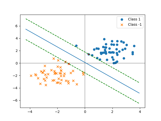
A key point is that \(\mathbf{\alpha}\) will be a sparse vector since there are only two points that are taken into consideration to construct the hyperplane.
Kernels.
def _RBF_kernel(X1, X2, gamma = 1):
        m, d1 = X1.shape
        n, d2 = X2.shape

        # Compute pairwise squared Euclidean distances
        # This comes from the fact that ||x - y||^2 = ||x||^2 + ||y||^2 - 2<x, y>
        # Which is the analogous to the elemental identity (a - b)^2 = a^2 + b^2 - 2ab
        dist_sq = np.sum(X1**2, axis=1).reshape((m, 1)) + np.sum(X2**2, axis=1) - 2 * np.dot(X1, X2.T)

        # Compute RBF kernel matrix
        K = np.exp(-gamma * dist_sq)

        return K

    def kernel(X1, X2):
        """
        RBF kernel
        """
        return _RBF_kernel(X1, X2)
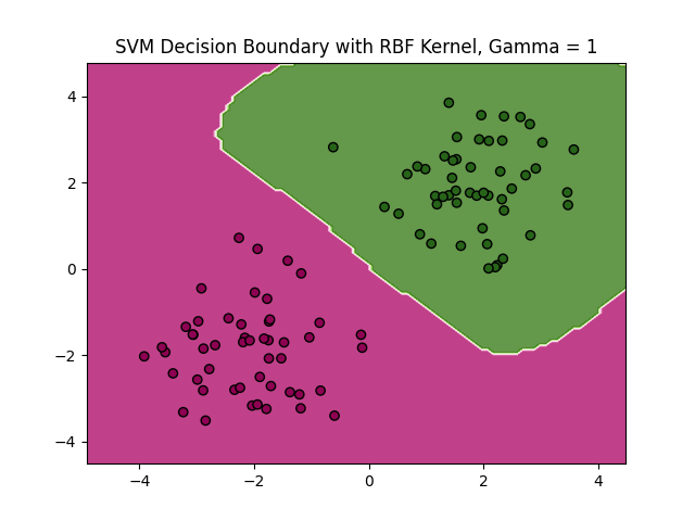
We can go one step further and enrich the basis of our data with an infinite dimensional basis, using, for example, the Radial Basis Function (RBF) (check this out). Since we construct a “similarity” matrix with the inner products of the data points, we could have any number of dimensions in those data points if we can find a way of computing the inner product (which is the definition of a Hilbert space). In the case of the RBF this is given by:
\[K(\mathbf{x}_i, \mathbf{x}_j) = \exp(-\gamma ||\mathbf{x}_i - \mathbf{x}_j||^2)\]Where \(\gamma\) is a hyperparameter. Which results in:
Some comments on how this is made are relevant since it is not immediate how to make predictions when using a kernel. It implies that we can only work with \(\mathbf{X}\mathbf{X}^T\) forms. We cannot explicitly compute the weights of the hyperplane (we can, and need, compute the bias, however). Luckily this is not a problem since, from the definition of the weights:
\[\mathbf{\beta} = \sum_{i=1}^n \alpha_i y_i \mathbf{x}_i\]we can see that this is just a sum over the rows of the dataset weighted by the Lagrange multipliers. This means that \(\mathbf{\beta}\) is just a weighted sum of the support vectors (\(\alpha_i \neq 0\)). Since then we can compute the predictions as:
\[\hat{y} = \text{sign}(\beta \mathbf{x}_j^T + \beta_0)\]Plugging in the definition of \(\beta\) we get:
\[\hat{y} = \text{sign}(\sum_{i=1}^n \alpha_i y_i \mathbf{x}_i \mathbf{x}_j^T + \beta_0)\]which we can turn into:
\[\hat{y} = \text{sign}(\sum_{i=1}^n \alpha_i y_i K(\mathbf{x}_i, \mathbf{x}_j) + \beta_0)\]for \(K\) being the kernel function. So we can calculate the bias term as:
\[\beta_0 = \frac{1}{N_S} \sum_{i \in S} (y_i - \sum_{j \in S} \alpha_j y_j K(\mathbf{x}_i, \mathbf{x}_j))\]using the mean over the support vectors (or just using one support vector, as in the code). The class predictions then;
\[\hat{y} = \text{sign}(\sum_{i=1}^n \alpha_i y_i K(\mathbf{x}_i, \mathbf{x}_j) + \beta_0)\]
    b_kernel = y[idx_support_vectors[0]] - np.sum((alphas * y).reshape(-1, 1) * kernel(X, X), axis=0)[idx_support_vectors[0]]
    prediction_fun = lambda X_test: np.sign(np.sum((alphas * y).reshape(-1, 1) * kernel(X, X_test), axis=0) + b_kernel)
Final comments.
The reflection about “modern” ML and traditional ML, representation learning vs kernels will have to wait until the end of the SVMs blog.
Here we learned about the optimal separating hyperplane problem, which is the basis of SVMs. We saw how to formulate the problem and how to solve it. We also saw how to use kernels to enrich the basis of our data and how to make predictions with them. That’s it for now!