Diffusion Models I. Approximating the gradient of the data distribution.
Diffusion models are another approach to generative modelling. The algorithm became popular with the release of Dalle-2 and Stable Diffusion. However, the underlying idea has been around for some time already.
In these notes, I will not focus on the details of the current SOTA algorithms but on the mathematical foundations of the idea. I will not describe conditional (image) generation. I will focus on sampling from the unknown probability distribution of a given dataset, first 2D and finally MNIST. My idea here is to provide an intuition of how this stuff works. For a more rigorous treatment check the references!
As an exercise I translated the pytorch code I found to tensorflow so all code here is in the latter. (I am using python 3.9.13)
These notes are (mostly) based on:
[1] This excellent repository: https://github.com/acids-ircam/diffusion_models
[2] This awesome article: https://arxiv.org/abs/2208.11970
[3] The work from Yang Song, who accompanies his research with super helpful blog posts: https://yang-song.net/blog/2019/ssm/, https://yang-song.net/blog/2021/score/ with the paper https://arxiv.org/abs/1907.05600.
[4] Some classic papers on the topic: https://arxiv.org/pdf/2006.11239.pdf, https://www.jmlr.org/papers/volume6/hyvarinen05a/hyvarinen05a.pdf, https://www.iro.umontreal.ca/~vincentp/Publications/smdae_techreport.pdf, https://arxiv.org/abs/1505.04597, chapter 5 Deep Learning book, RefineNet
[5] Some other blogposts like: https://lilianweng.github.io/posts/2021-07-11-diffusion-models/
Introduction
The name diffusion already gives a clue about the underlying idea: Reversing a diffusion process. To do so, we construct a function that can go from pure noise (the endpoint of the diffusion process) to the original coherently structured substance (the original point). In this sense, going from noise to coherent data, diffusion models are similar to GAN, but the similarities end there.
Another way of looking at this, motivated by the score based modelling point of view, is the idea of “navigating” a high dimensional space towards the areas where the coherence (w.r.t our data) within the dimensions is maximized. Or, what is the same, climbing a high dimensional probability distribution towards the peak areas. To clarify, high probability regions (the peaks) in this space are where the combination of the dimensions is more likely to render an observation belonging to our dataset. This is, gradient ascent w.r.t. the data distribution, starting from noise (random initialization) and generating an image. This is illustrated in the next GIF (which will be generated from scratch in these notes):
Surprisingly enough, it is possible to estimate gradients of a dataset even when we do not have an explicit probability distribution (if we had it there would be no point in doing this anyway).
As a metaphor, what we are going to train here is the compass of the “navigators”, a model that gives us the gradient w.r.t the data distribution at any given point such that we can find our way towards high probability regions.
How can we estimate the gradient of a dataset? Let’s get to it!
Estimating the gradient of a dataset:
Imports and the data:
import numpy as np
import matplotlib as mpl
import matplotlib.pyplot as plt
from sklearn import datasets
import tensorflow as tf
from tensorflow import keras
from tensorflow.keras import layers
from tqdm import tqdm
import tensorflow_addons as tfa
plt.style.use('Solarize_Light2')
def get_batch(size, noise = 0.05, type = 'moons'):
if type == 'moons':
sample = datasets.make_moons(n_samples=size, noise=noise)[0]
else:
sample = datasets.make_circles(n_samples=size, factor=0.5, noise= noise)[0]
return sample
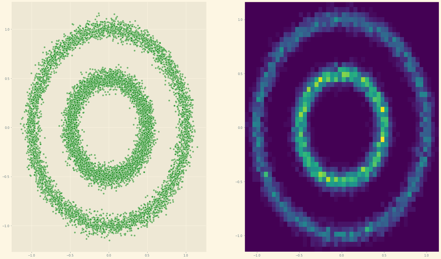
data = get_batch(10**4, type = '')
fig, (ax1, ax2) = plt.subplots(1, 2, figsize=(25, 15))
ax1.scatter(*data.T, alpha = 0.5, color = 'green', edgecolor = 'white', s = 40)
ax2.hist2d(*data.T, bins = 50);
For an unknown probability distribution \(p(x)\) we want to estimate \(\nabla \log p(x)\). So we can frame this as a regression problem with something like:
$$\frac{1}{2}\mathop{\mathbb{E}}_{x \sim p(x)}[|| \mathcal{F}_{\theta} - \nabla \log p(x)||²]$$
Being \(\mathcal{F}_{\theta}\) a very flexible function, like a neural network with parameters \(\theta\).
Yeah, but we don’t know \(p(x)\)! It turns out (using integration by parts and some reasonable assumptions) that the above equation can be reformulated as:
$$\mathop{\mathbb{E}}_{x \sim p(x)} \bigg[\text{tr}(\nabla_x \mathcal{F}_{\theta}(x)) + \frac{1}{2}||\mathcal{F}_{\theta}(x)||^2 \bigg]$$
(The trace arises in the multidimensional version.)
Which does not have any \(p(x)\) inside. Now, this, called (vanilla) score based generative modelling can already be used.
Let’s check if we can approximate the gradient of the above 2D circle’s dataset.
First, let’s define our \(\mathcal{F}_{\theta}(x)\) using a fully conected network:
# The gradient
# Now, this takes the point (x_1, x_2) and returns the gradient w.r.t. (x_1, x_2) at that point.
F_model = tf.keras.Sequential([
    layers.Dense(128, input_shape = (2, ), activation= 'linear'),
    layers.Dense(128, activation= 'gelu'),
    layers.Dense(64, activation= 'gelu'),
    layers.Dense(32, activation= 'gelu'),
    layers.Dense(2, activation= 'linear') # TWO DIMENSIONS!
])
And \(\nabla_x \mathcal{F}_{\theta}(x)\):
# Generate the Hessian
@tf.function
def Hessian(F, x):
    '''
    Computes jacobian of the gradient (F_model) w.r.t x.
    :param F: function R^N -> R^N
    :param x: tensor of shape [B, N]
    :return: Jacobian matrix of shape [B, N, N]

    '''
    with tf.GradientTape() as tape:
        tape.watch(x)
        my_gradient = F(x)
        hessian = tape.batch_jacobian(my_gradient, x)

    return hessian
Notice that the derivatives are w.r.t the data x (not the parameters of F_model network):
Nice! then we only need to compute the loss, as we specified above:
# Now, I have the Jacobian (the gradient) (B, 2) and the Hessian (B, 2, 2)
def score_matching(F, x):
    gradient = F(x)

    # Jacobian part
    norm_gradient = (tf.norm(gradient, axis = 1) ** 2) /2
    # Hessian part
    hessian = Hessian(F, x)

    tr_hessian = tf.cast(tf.linalg.trace(hessian), dtype = tf.float32)

    return tf.math.reduce_mean(tr_hessian + norm_gradient, axis = -1)
And training loop:
# Now training loop
optimizer = keras.optimizers.Adam(learning_rate= 1e-4)

loss_l = []

for t in range(2500): #Epochs
    with tf.GradientTape() as tape:
        loss = score_matching(F_model, data)

        if len(loss_l) > 1:
            if loss_l[-2] < loss_l[-1]: # trivial early stopping
                break

        model_grads = tape.gradient(loss, F_model.trainable_weights)

        optimizer.apply_gradients(zip(model_grads, F_model.trainable_weights))


        loss_l.append(loss)
        if ((t % 100) == 0):
            print(loss_l[-1])

F_model.save_weights('./Vanilla_score_weights.h5')
We now can plot the gradients that out F_model estimates:
def plot_gradients(model, data, plot_scatter = True):
    xx = np.stack(np.meshgrid(np.linspace(-1.5, 2.0, 50), np.linspace(-1.5, 2.0, 50)), axis = -1).reshape(-1, 2)
    scores = model(xx).numpy() # the gradients w.r.t each data point!
    # This is, how much the DENSITY OF THE DATA increases at a given point of the xx (meshgrid)

    # Now that stuff is not good to visualize. Some scaling to make a nice plot:
    scores_nrom = np.linalg.norm(scores, axis = -1, ord = 2, keepdims = True)
    scores_log1p = scores / (scores_nrom + 1e-9) * np.log1p(scores_nrom)
    plt.figure(figsize=(16,12))
    if (plot_scatter):
        plt.scatter(*data.T, alpha=0.3, color='red', edgecolor='white', s=40)
    plt.quiver(*xx.T, *scores_log1p.T, width=0.002, color='black')
    plt.xlim(-1.5, 2.0)
    plt.ylim(-1.5, 2.0)

plot_gradients(F_model, data)
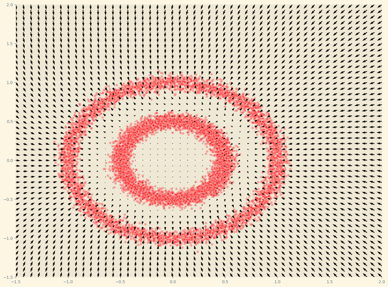
As we can see, this surprisingly works! That’s far from evident just looking at the loss function! To sample we can use a combination of the gradient and some noise: langevin dynamics.
def langevin_dynamics(F, x, n_steps, eps = 0.7e-2, decay = .9, temperature = 1):
    # Just a naive langevin dynamics "sampler"
    x_sequence = [x]
    for s in range(n_steps):
        z_t = np.random.normal(size = x.shape)
        gradient = F(x).numpy()

        x = x + eps * (gradient +  (temperature * z_t ))
        x_sequence.append(x)
        eps *= decay

    return np.array(x_sequence).reshape(n_steps + 1, 2)
Now, there is a very important detail. This method does not work well in high-dimensional spaces, where most of the space is empty. This is especially relevant for images, which live in a low-dimensional manifold. In that case \(\log p(x)\) may become \(-\infty\). A way to solve this is to add noise to the data to fill the empty space and have reliable gradients everywhere. Solving the data sparsity problem in a high dimensional space through noise is one of the key ideas in Diffusion Models.
Now, while this is cool and I think helps in understanding the connection with the unknown \(p(x)\), there is even a more surprising, simpler and efficient approach. We can approximate the log “gradient” of the data distribution as the gradient of a Gaussian density
\[q_{\sigma}(\tilde{x}|x)\]with mean at \(x\) and standard deviation \(\sigma\) w.r.t. a noisy data point \(\tilde{x}\).
This makes intuitive sense, the “gradient” should point us towards a combination of parameters which renders a less noisy data point. This is called denoising score matching. Using Gaussian noise and a Gaussian density as the kernel, the loss function looks like:
$$Loss(\theta| \sigma) = \mathop{\mathbb{E}}_{x \sim p(x)} \bigg[\frac{1}{2}\bigg|\bigg|\mathcal{F}_{\theta}(\tilde{x}, \sigma) - \frac{x - \tilde{x}}{\sigma^2} \bigg|\bigg|^2_2 \bigg]$$
Because:
$$\frac{\mathbb{d}\log q_{\sigma}(\tilde{x}|x)}{\mathbb{d}\tilde{x}} = \frac{x- \tilde{x}}{\sigma^2}$$.
Same as before, however, we want a reliable “gradient” everywhere. The solution here is to add different levels of noise \(\sigma\):
# Different sigma values
sigma_begin = 1
sigma_end = 0.01
num_noises = 10
sigmas = np.exp(np.linspace(np.log(sigma_begin), np.log(sigma_end), num_noises))
plt.plot(sigmas)
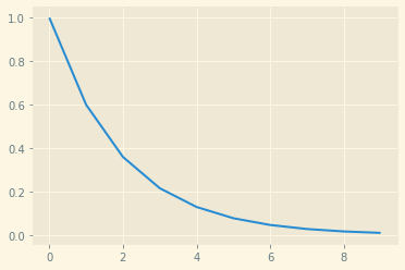
And this looks like:
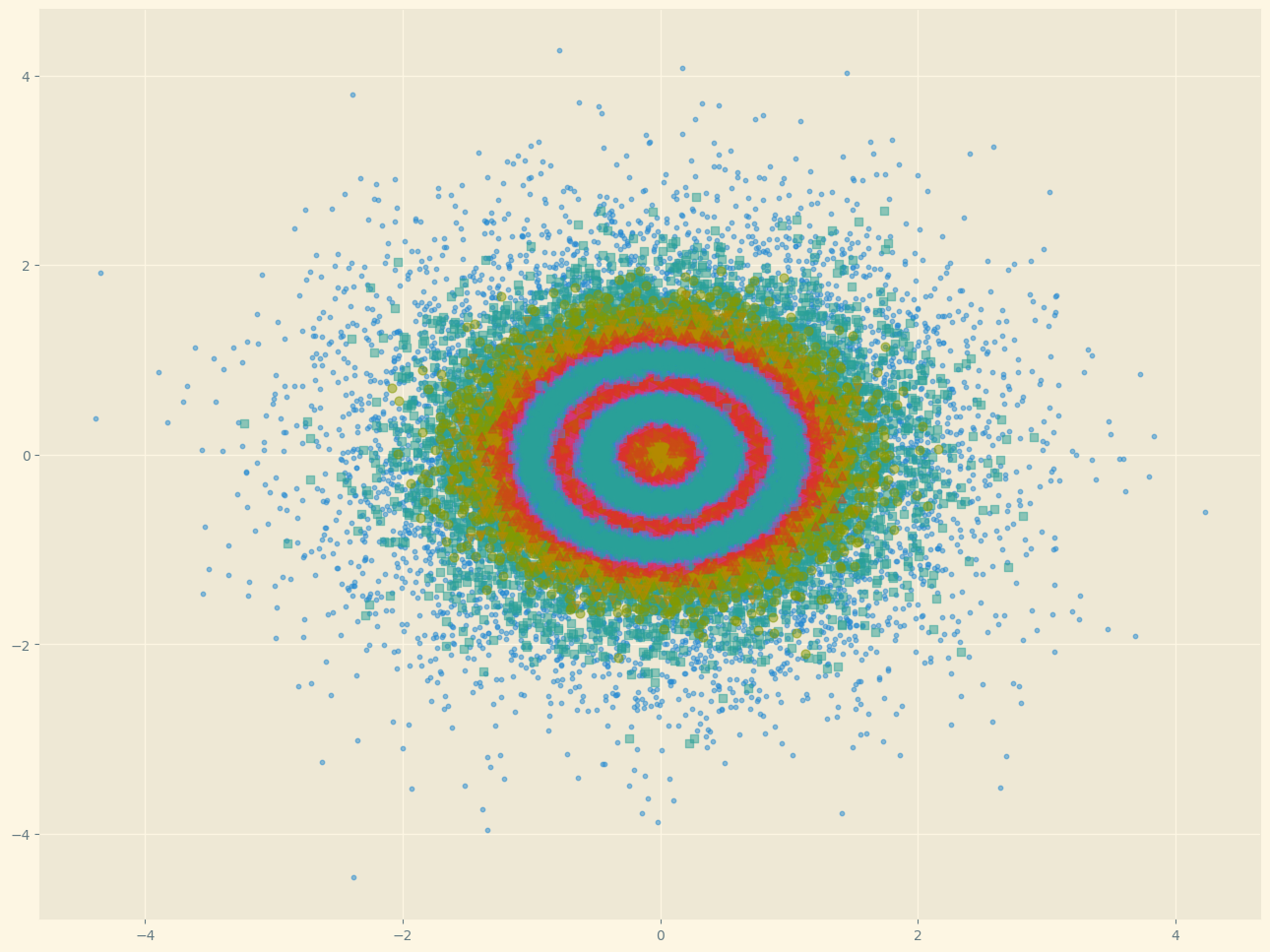
Here we have the noise added to the initial data and plotted on top in different color/shape.
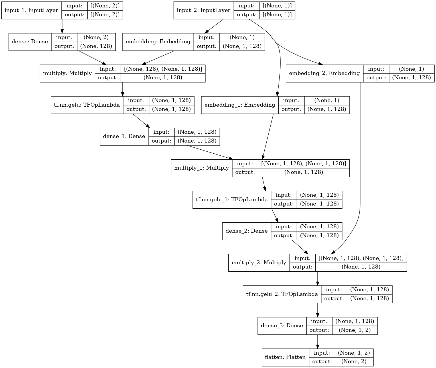
This works best if we let our model know (our approximation to the gradient) at which noise level \(\sigma\) we are. So this time our model (our fully connected NN) will also take an embedding of the \(\sigma\) level. And we will insist on it! Feeding a representation of the noise level index at every layer.
Input_data = keras.Input(shape=(2,))
labels_input = keras.Input(shape=(1,))

d = layers.Dense(128, activation= 'linear')(Input_data)
l = tf.keras.layers.Embedding(num_noises, 128)(labels_input)

d = keras.layers.Multiply()([d, l])
d = tf.keras.activations.gelu(d)

for i in (128, 128):
    d = layers.Dense(i, activation= 'linear')(d)
    l =  tf.keras.layers.Embedding(num_noises, i)(labels_input)

    d = keras.layers.Multiply()([d, l])
    d = tf.keras.activations.gelu(d)

output = keras.layers.Dense(2)(d)
output = keras.layers.Flatten()(output)

F_model = keras.Model([Input_data, labels_input], output)
Which is already looking relatively fancy! And this is just 2D!
And we generate some \(\sigma\) levels (indexes) to use during training:
labels = np.random.randint(0, num_noises, data.shape[0])
Now we are ready to write down our Noise Conditional Loss function:
def conditional_noise_loss(F, x, labels = labels, sigmas = sigmas):

    used_sigmas = sigmas[labels][..., np.newaxis]

    # Generate noise for a given level (label)
    noise = np.random.normal(size = x.shape) * used_sigmas

    perturbed_x = x + noise

    # \frac{x - \tilde{x}}{\sigma^2}
    target =  tf.constant((data - perturbed_x) / (used_sigmas ** 2), dtype =tf.float32)

    # Our approximation to the gradient now takes 2 inputs:
        # The noisy x.
        # The noise (index) level.
    gradient = F([perturbed_x, labels]) # takes the label as embedding!

    loss = 1/2 * (tf.norm(gradient - target, axis = 1)) * used_sigmas ** 2

    return tf.math.reduce_mean(loss)
And we can train this:
# Now training loop
optimizer = keras.optimizers.Adam(learning_rate= 1e-3)

loss_l = []
epochs = tqdm(range(5000))
for t in epochs:
    with tf.GradientTape() as tape:
        loss = conditional_noise_loss(F_model, data)

        model_grads = tape.gradient(loss, F_model.trainable_weights)

        optimizer.apply_gradients(zip(model_grads, F_model.trainable_weights))


        loss_l.append(loss)
        epochs.set_description("Loss: %s" % loss_l[-1].numpy())

F_model.save_weights('./Denoising_conditional_weights.h5')
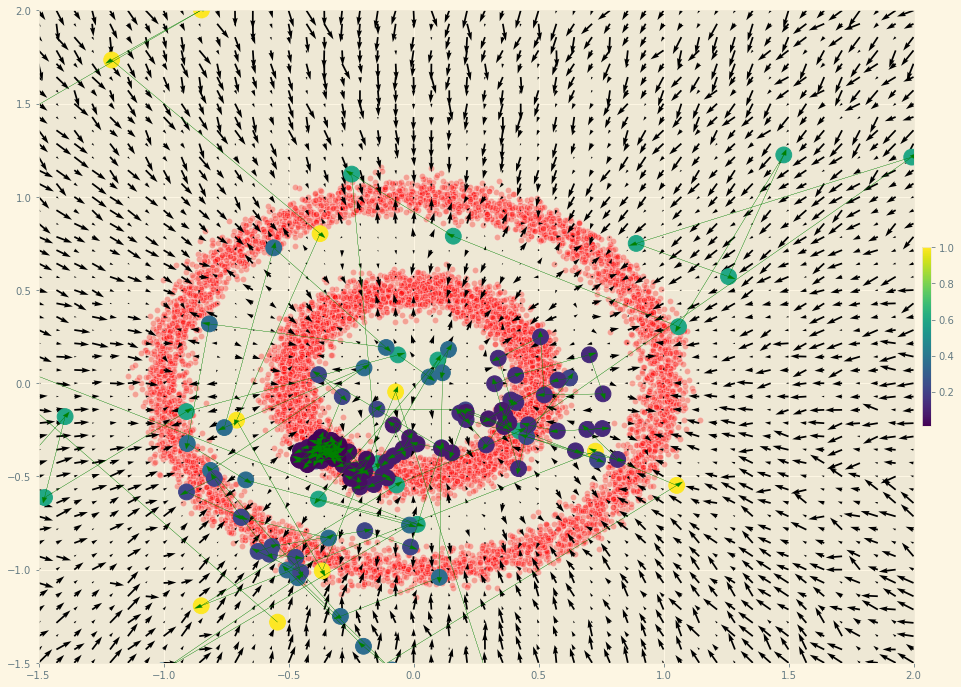
And once it is done we can again visualize the gradients:
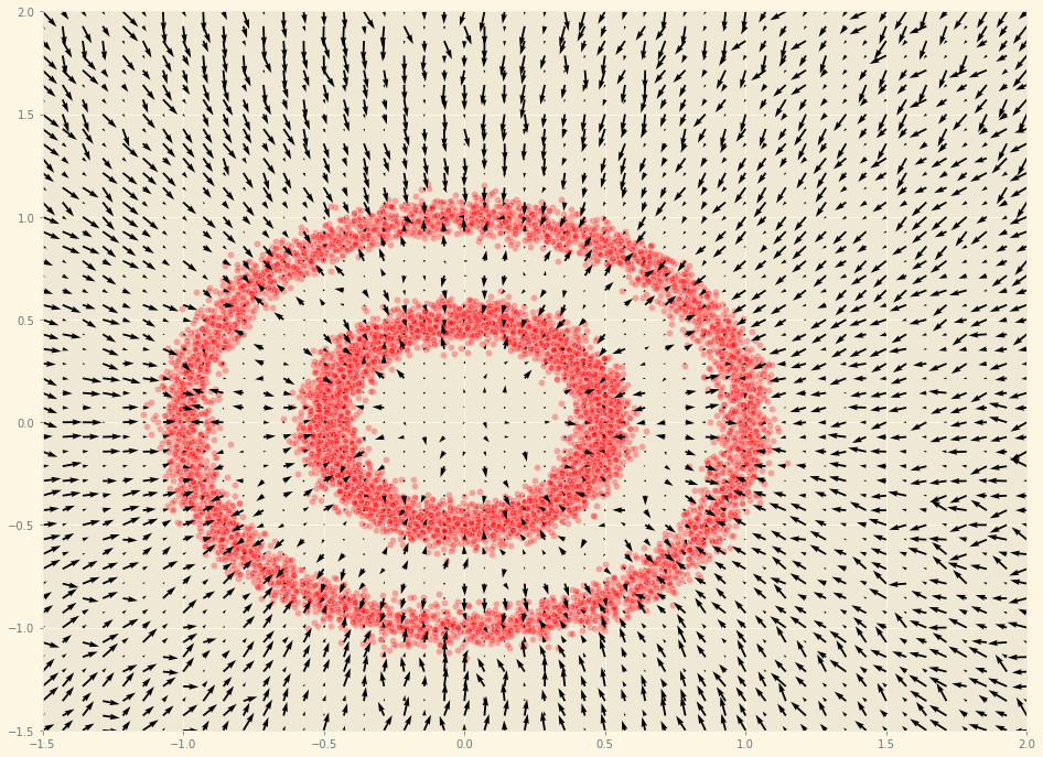
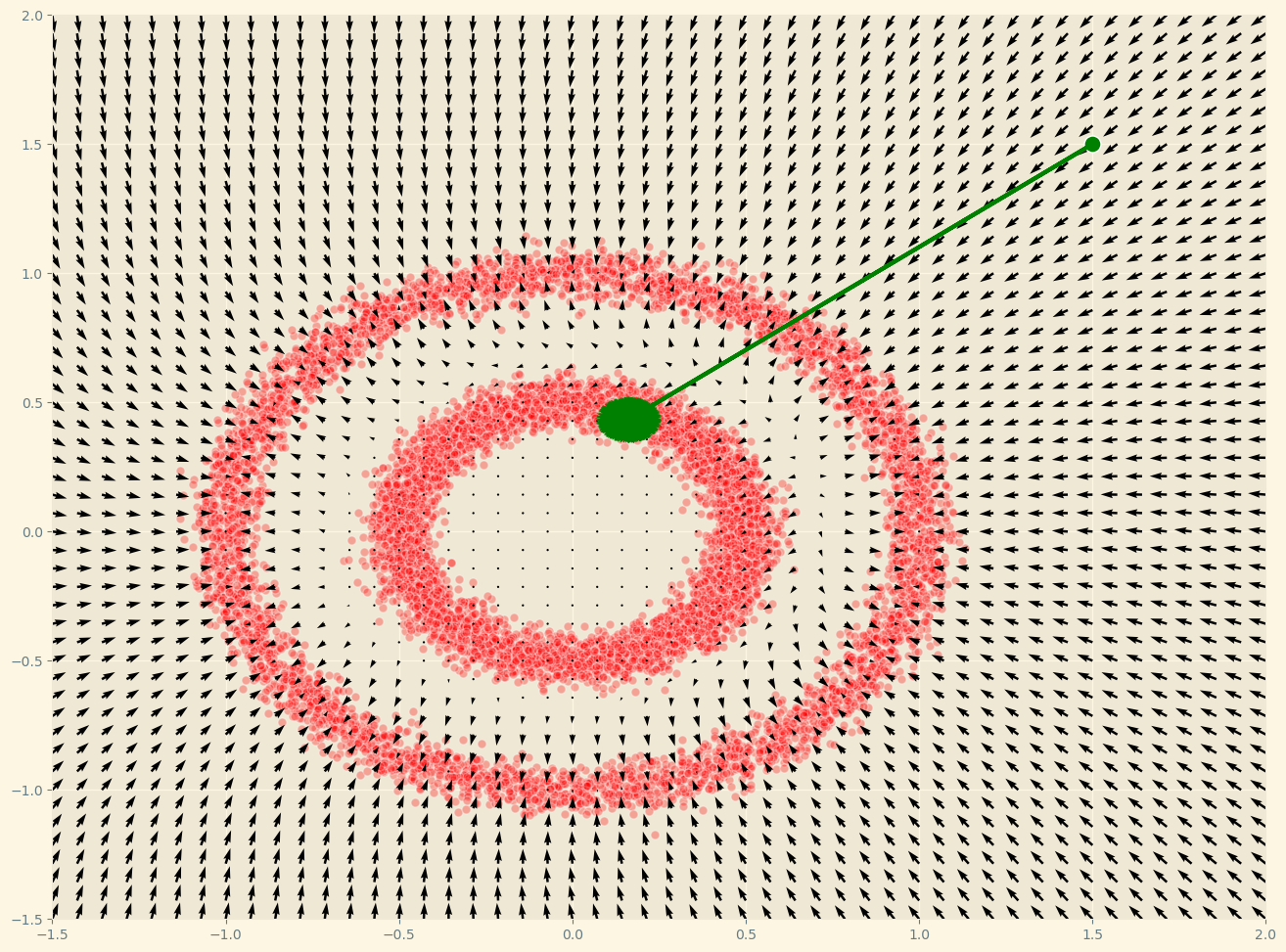
And to sample, we can use a fancier version of the ‘langevin_dynamics’ function we used before. It does the same but looping over different noise levels.
def ald_sampling(F, sigmas, num_noises, iter, step_size):
    '''
    Sampling and visualization.

    '''
    plot_gradients(F_model, data) # Plot distribution landscape

    x_t = np.random.normal(size = (1, 2)) # Initial sample

    samples = [] # Placeholder

    # Loop over noise levels:
    for noise_level in range(num_noises):
        alpha = step_size * (sigmas[noise_level]**2 / sigmas[-1]**2)
        # noise level inner sampling:
        for t in range(iter):
            z = np.random.normal(size = (1, 2))
            gradient = F([x_t, np.array([[noise_level]])]).numpy()

            x_t = x_t + (alpha/2) * gradient + np.sqrt(alpha) * z
            samples.append(np.ravel(x_t))

    # Plot (given noise level) samples
    color = np.array([[i] * iter for i in sigmas]).ravel()

    plt.scatter(*np.array(samples).T, s=250, c = color)

    samples = np.array(samples)
    # Draw arrrows
    deltas = (samples[1:] - samples[:-1]) # Difference

    for i, arrow in enumerate(deltas):
        plt.arrow(samples[i,0], samples[i,1], arrow[0], arrow[1],
                    width=1e-4, head_width=2e-2, color="green", linewidth=0.2)
    plt.colorbar(fraction=0.01, pad=0.01)
    plt.show()
    return samples

samples = ald_sampling(F_model, sigmas, num_noises, 20, 0.0001)
Now we can see how when the level of noise decreases the samples converge to the actual data distribution. The colour indicates the amount of noise, from maximum (yellow) to minimum (purple).
Estimating the gradient for MNIST:
MNIST is way more challenging, but the underlying principles are the same!
Data loading and scaling:
def scale_image(image):
    return (image - (255/2)) / (255/2) # -1 to 1 to make it easier

data_mnist = keras.datasets.mnist.load_data(path="mnist.npz")[0][0]
data_mnist = scale_image(data_mnist[..., np.newaxis])
And now… we really need to go fancy with the model. An arbitrary network does not work, we need something with a proper inductive bias. Since we are concerned with the gradient at the pixel level (each of our dimensions) but still need to take information over the whole picture, a network designed for image segmentation is ideal. An option is RefineNet (the images are from the paper).
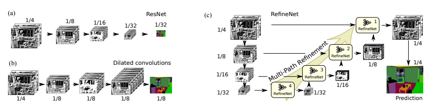
The idea is to first downsample the data using a ResNet to 1/4, 1/8, 1/16 and 1/32 (in our case we begin in 1/1). The stride is typically set to 2, thus reducing the feature map resolution to one-half when passing from one block to the next.
After, it applies a multi path refinement (as shown in the image). The key point here is that the downsampling allows us to get general information about the picture while at the same time, eventually, focusing at the pixel level. Each RefineNet block takes a representation of the downsampled version and a higher resolution version until, in our case, reaching the pixel level
Nevertheless, there is still the issue of how to encode the \(\sigma\) level information. One option is to use “conditional instance normalization”. Instance normalization consists basically on normalizing the feature maps per image.
Now, what this does is: Let \(\mu_k\) and \(s_k\) denote mean and std of the k-th feature map of x (an image).
\[z_k = \gamma[i, k]\frac{x_k - \mu_k}{s_k} + \beta[i, k]\]Where \(\gamma\) and \(\beta\) are learnable parameters. These parameters are embeddings of the noise level. The dimensionality of the embedding is such that there is a scalar for each channel. Hence, given k, \(\gamma\) and \(\beta\) are scalars. Basically, we are doing sort of the same as before, scaling the output of the convolutional layers based on the embedding of the noise level.
Let’s code it. First instance normalization:
class CIN(tf.keras.layers.Layer):
    def __init__(self, num_noises, num_features):
        super().__init__()
        self.num_features = num_features
        self.num_noises = num_noises
        self.instance_norm = tfa.layers.InstanceNormalization()

        self.gamma = tf.keras.layers.Embedding(input_dim = self.num_noises,
                                            output_dim = self.num_features,
                                            embeddings_initializer = tf.keras.initializers.RandomNormal(1., 0.02))

        self.beta = tf.keras.layers.Embedding(input_dim = self.num_noises,
                                            output_dim = self.num_features,
                                            embeddings_initializer = 'Zeros')

    def call(self, image, noise_level):

        image_norm = self.instance_norm(image) # (B, height, width, num_features)

        # Scalars
        my_gamma = tf.expand_dims(self.gamma(noise_level), axis = 1) # (B, 1, 1  num_features)

        my_beta = tf.expand_dims(self.beta(noise_level), axis = 1)# (B, 1, 1, num_features)

        z = my_gamma * image_norm + my_beta # (B, height, width, num_features)

        return z
Let’s construct a ResNet:
# norm -> non-linear -> conv -> norm -> non-linear -> conv -> Downsample by 2

class ResNetBlock(tf.keras.layers.Layer):
    def __init__(self, output_features, num_noises, downsampling = True):
        super().__init__()

        self.downsampling = downsampling

        self.act = tf.keras.layers.ELU()

        self.embd1 = CIN(num_noises, output_features)
        self.embd2 = CIN(num_noises, output_features)

        self.conv1 = tf.keras.layers.Conv2D(output_features,
                                                        kernel_size = 3,
                                                        padding = 'SAME')

        self.conv2 = tf.keras.layers.Conv2D(output_features,
                                                        kernel_size = 3,
                                                        padding = 'SAME')

        self.down =  tf.keras.layers.Conv2D(output_features,
                                                        kernel_size = 3,
                                                        strides = 2,
                                                        padding = 'SAME')

    def call(self, image, noise_level):

        h = self.embd1(image, noise_level)
        h = self.act(h)
        h = self.conv1(h)

        h = self.embd2(h, noise_level)
        h = self.act(h)
        h = self.conv2(h)

        if self.downsampling:
            return self.down(image + h)
        else:
            return image + h
Ok, now let’s deal with RefineNet:
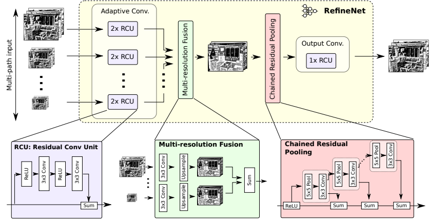
It consists of a residual convolutional unit, multi-resolution fusion and chained residual pooling.
# Residual convolutional Unit
class RCU(tf.keras.layers.Layer):
    def __init__(self, input_features, num_noises):
        super().__init__()

        self.Embedding1 = CIN(num_noises, input_features)
        self.Convolution1 = tf.keras.layers.Conv2D(input_features,
                                                    kernel_size = 3,
                                                    activation = 'ELU',
                                                    padding = 'SAME')

        self.Embedding2 = CIN(num_noises, input_features)
        self.Convolution2 = tf.keras.layers.Conv2D(input_features,
                                                    kernel_size = 3,
                                                    padding = 'SAME')

        self.first_act = tf.keras.layers.ELU()

    def call(self, image, noise_level):

        res = image

        x = self.first_act(image)
        x = self.Embedding1(x, noise_level)
        x = self.Convolution1(x)
        x = self.Embedding2(x, noise_level)
        x = self.Convolution2(x)


        return res + x

# Now the multi resolution thing:
class MRF(tf.keras.layers.Layer):
    def __init__(self, im_in, input_features, num_noises, shape_target):
        super().__init__()

        self.shape_target = shape_target
        self.im_in = im_in
        self.embeddings = []
        self.Conv = []


        for i in range(im_in):
            self.embeddings.append(CIN(num_noises, input_features))
            self.Conv.append(tf.keras.layers.Conv2D(input_features,
                                                        kernel_size = 3,
                                                        padding = 'SAME'))


    def call(self, images, noise_level):


        if  self.im_in == 1:
            h = self.embeddings[0](images[0], noise_level)
            h = self.Conv[0](h)

            h = tf.image.resize(h, self.shape_target[:2])

            return h

        else:

            h1 = self.embeddings[0](images[0], noise_level)
            h1 = self.Conv[0](h1)

            h1 = tf.image.resize(h1, self.shape_target[:2]) # Resizes, if needed, to target
            #Upsmaples using bilinear interpolation
            h2 = self.embeddings[1](images[1], noise_level)
            h2 = self.Conv[1](h2)

            h2 = tf.image.resize(h2, self.shape_target[:2])
            sums = h1 + h2

            return sums

# Chained residual pooling
class CRP(tf.keras.layers.Layer):
    def __init__(self, input_features, num_noises, n_blocks = 2):
        super().__init__()

        self.embeddings = []
        self.conv = []
        self.avg_pool = []

        self.n_blocks = n_blocks
        for i in range(n_blocks):
            self.embeddings.append(CIN(num_noises, input_features))
            self.avg_pool.append(tf.keras.layers.AveragePooling2D(pool_size = 5,
                                                                  padding = 'SAME',
                                                                  strides = 1))
            self.conv.append(tf.keras.layers.Conv2D(input_features,
                                                        kernel_size = 3,
                                                        padding = 'SAME'))

            self.first_act = tf.keras.layers.ELU()

    def call(self, image, noise_level):

        x = self.first_act(image)

        sum = x

        for i in range(self.n_blocks):
            x = self.embeddings[i](x, noise_level)
            x = self.avg_pool[i](x)
            x = self.conv[i](x)

            sum = x + sum

        return sum
So a block of RefineNet:
class RefineNetBlock(tf.keras.layers.Layer):
    def __init__(self, im_in, input_features, num_noises, shape_target):
        super().__init__()

        self.RCUBig1 = RCU(input_features, num_noises)
        self.RCUBig2 = RCU(input_features, num_noises)

        if im_in == 2:
            self.RCUSmall1 = RCU(input_features, num_noises)
            self.RCUSmall2 = RCU(input_features, num_noises)

        self.MRF = MRF(im_in, input_features, num_noises, shape_target)
        self.CRP = CRP(input_features, num_noises)

        self.final_conv = RCU(input_features, num_noises)

    def call(self, image_big, image_small, noise_level):

        image_big_processed = self.RCUBig1(image_big, noise_level)
        image_big_processed = self.RCUBig2(image_big_processed, noise_level)

        if image_small is not None:
            image_small_processed = self.RCUSmall1(image_small, noise_level)
            image_small_processed = self.RCUSmall2(image_small_processed, noise_level)

            x = self.MRF([image_big_processed, image_small_processed], noise_level)
        else:
            x = self.MRF([image_big_processed], noise_level)

        x = self.CRP(x, noise_level)
        x = self.final_conv(x, noise_level)

        return x
Indeed, the network is quite complex (and this is nothing!). Let’s put everything together.
Naturally, we do not want to work with the image in 1/4 but in 1/1 so in the first ResNet we do not downsample the output. Hence, the downsampling process goes (28, 28) -> (14, 14) -> (7, 7) -> (4, 4). We do not have to worry about the upsampling process since it is taken care of by the bilinear interpolation, which is much more flexible than deconvolutions.
The only thing left is to construct the model and train! All the rest is the same as before in the 2D case!
def make_model(n_filters, num_noises):
    Input_image = keras.Input(shape=(28, 28, 1))
    Input_label = keras.Input(shape=(1,))

    res1 = ResNetBlock(n_filters, num_noises= num_noises, downsampling = False)(Input_image, Input_label)
    res2 = ResNetBlock(n_filters, num_noises= num_noises)(res1, Input_label)
    res3 = ResNetBlock(n_filters, num_noises= num_noises)(res2, Input_label)
    res4 = ResNetBlock(n_filters, num_noises= num_noises)(res3, Input_label)

    RefineNet_4 = RefineNetBlock(im_in= 1,
                                input_features = n_filters,
                                num_noises= num_noises,
                                shape_target= (4, 4, 1))(image_big = res4,
                                                        image_small = None,
                                                        noise_level = Input_label)

    RefineNet_3 = RefineNetBlock(im_in= 2,
                                input_features = n_filters,
                                num_noises= num_noises,
                                shape_target= (7, 7, 1))(image_big = res3,
                                                        image_small = RefineNet_4,
                                                        noise_level = Input_label)

    RefineNet_2 = RefineNetBlock(im_in= 2,
                                input_features = n_filters,
                                num_noises= num_noises,
                                shape_target= (14, 14, 1))(image_big = res2,
                                                        image_small = RefineNet_3,
                                                        noise_level = Input_label)

    RefineNet_1 = RefineNetBlock(im_in= 2,
                                input_features = n_filters,
                                num_noises= num_noises,
                                shape_target= (28, 28, 1))(image_big = res1,
                                                        image_small = RefineNet_2,
                                                        noise_level = Input_label)


    #And eventually just a linear combination of the features to map the dimensionality of the input:

    final_conv = tf.keras.layers.Conv2D(1, 1, strides= 1)(RefineNet_1)

    F_model = tf.keras.Model([Input_image, Input_label], final_conv)

    return F_model

F_model = make_model(64, 10)
This takes a bit more to train so the weights are available here
The training loop:
# Now training loop
optimizer = keras.optimizers.Adam(learning_rate= 1e-3)

loss_l = []
batch_size = 32

# Epochs loop
for t in range(50):
    epoch_loss = []
    # Batches loop:
    for b in tqdm(range(0, (data_mnist.shape[0] - batch_size), batch_size)):

        data = data_mnist[b: b + batch_size]
        loss_batch = []

        labels = np.random.randint(0, num_noises, data.shape[0])

        with tf.GradientTape() as tape:
            loss = conditional_noise_loss(F_model, data, labels = labels)
            loss_batch.append(loss)


            model_grads = tape.gradient(loss, F_model.trainable_weights)

            optimizer.apply_gradients(zip(model_grads, F_model.trainable_weights))


    loss_l.append(np.mean(loss_batch))
And a sampler adapted to the MNIST:
def ald_sampling_mnist(F, sigmas, num_noises, iter, step_size, num_samples = 10):

    x_t = np.random.uniform(low = -1., high = 1, size = (num_samples, 28, 28, 1)) # Initial sample

    samples = [] # Placeholder

    # Loop over noise levels:
    for noise_level in tqdm(range(num_noises)):
        #print(f'noise level {noise_level}')
        alpha = step_size * (sigmas[noise_level]**2 / sigmas[-1]**2)
        # noise level inner sampling:
        for t in range(iter):
            z = np.random.normal(size = (num_samples, 28, 28, 1))
            gradient = F([x_t, np.array([[noise_level] * num_samples]).T]).numpy()

            x_t = x_t + (alpha/2) * gradient + np.sqrt(alpha) * z
            samples.append(x_t)

    return samples
Run it:
iter = 100
num_samples = 64
samples = ald_sampling_mnist(F_model, sigmas, num_noises, iter = iter, step_size = 2e-5, num_samples = num_samples)
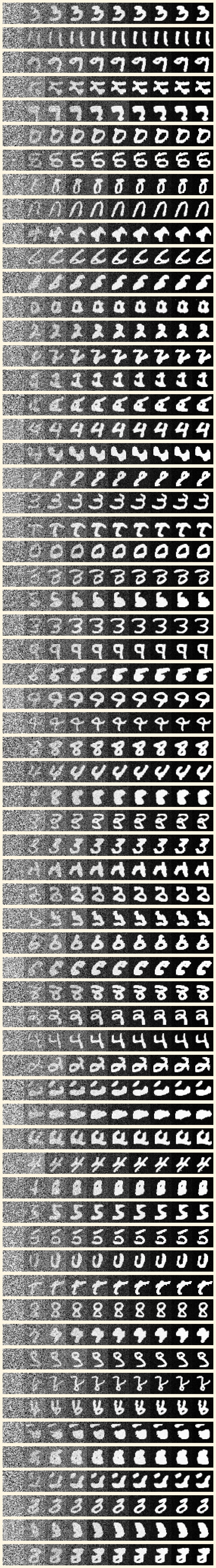
And now some plotting…
plt.figure(figsize=(10, int(num_samples * 1.2)))

for row in range(samples[0].shape[0]):
    for j, i in enumerate(range(0, len(samples), iter)):
        plt.subplot(samples[0].shape[0], len(samples) // iter, 1 + j + row * (len(samples) // iter))
        plt.imshow(samples[i][row] * -1, interpolation='nearest', cmap='Greys')
        plt.grid(b=None)
        plt.axis('off')

plt.subplots_adjust(wspace=0, hspace=0)
plt.show()
What you see here is the sampling process. From noise to coherent images, following the process that we have described here. This is not different from the 2D example but is way cooler since you can see the sampler “navigating” this 28*28 dimensional space until it reaches a peak in the probability distribution of our data. Or what is the same, a coherent handwritten number? Having understood this, it is even more staggering the outputs of SOTA algorithms like Stable Diffusion. Amazing time to be alive isn’t it?
and this to generate the GIF!
from moviepy.editor import ImageSequenceClip

images = []
height = int(np.sqrt(samples[0].shape[0]))

for step in tqdm(range(0, len(samples), 5)):
    plt.figure(figsize=(8, 8))
    for i in range(samples[step].shape[0]):
        plt.subplot(height, height, 1 + i)
        plt.imshow(samples[step][i] * -1, interpolation='nearest', cmap='Greys')
        plt.grid(b=None)
        plt.axis('off')
    plt.subplots_adjust(wspace=0.05, hspace=0.05)
    plt.savefig(f'./Gif_folder/{step}.png')
    images.append(f'./Gif_folder/{step}.png')
    plt.close()

clip = ImageSequenceClip(images, fps = 50)
clip.write_gif('MNIST_SAMPLING.gif')
And that’s all for part 1. The next part is on the actual diffusion model, which is really similar but still has some differences.