Pendulum, equations of motion from first principles and solutions using ML.
References
These notes are based on:
[1] Hardvard notes on Lagrangian method
[2] Classical Mechanics: The Theoretical Minimum
[3] Deep learning for universal linear embeddings of nonlinear dynamics
Introduction
Lately I have been reading “Classical Mechanics: The theoretical minimum”. Since I mostly deal with purely data-driven approaches, I wanted to dive a bit into the first-principle derivation of predictive models.
Here I look into the simplest pendulum, a mass whose motion is restricted to a unit circle.
First I derive a differential equation in which we can study the motion of the pendulum. Then I solve this differential equation in a data-driven way (i.e. construct a function of \(t\) that returns the angle and velocity of the pendulum given some initial conditions) using a linear model on a coordinate system generated by an autoencoder.
Derivation of the potential energy from first principles
Potential energy is just the amount of work that is potentially stored. In this case it is clear that when the red ball is at the top of the circle (0,1) the potential energy is maximum. This is because we are assuming that the only acting force here is gravity, so the higher up, the more potential energy. Then, we can be sure that the total potential energy is proportional to the y coordinate.
\[V(\theta) = mg(1-\cos(\theta))\]For \(\theta\) being the angle between the black and red line (see above .gif). On \((0, 1)\) the potential energy is at is maximum since \(\cos(\pi) = -1.\) \(mg\) is the constant to which the potential energy is proportional. Intuitively, this should be how much is the pull of the force down (gravity, in earth \(9.8 m/s^2\)) and the mass of the ball (assumed to be 1).
So far I have only used the fact that, the higher up, the more potential energy.
Derivation of the kinetic energy from first principles
Assuming that the acceleration is constant (which makes sense because the force applied is constant), kinetic energy is defined as \(T(\theta) = \frac{1}{2}mv^2\). This comes from the sum of the work applied over distance, distance being \(d = \frac{1}{2}vt\) (assuming speed 0 at time 0, think of the area of a triangle) and work per unit of time being the increase of momentum, \(F = ma = m\frac{v}{t}\) because \(a\) is constant, so \(W = Fd = mad = \frac{1}{2}mv^2.\)
Surely, the velocity can be expressed as the change in the angle per unit of time so \(v = \dot{\theta}.\) Then the kinetic energy is \(T(\theta) = \frac{1}{2}m\dot{\theta}^2.\) Going down is indeed negative velocity (the angle is getting smaller).
Derivation of the equation of motion
Now, since the total energy is constant, I could use that to try to get the equation of motion. However, using the principle of stationary action is cooler. This is defined as the integral of all possible paths of the difference between kinetic and potential energy (why this works is a matter for further study…).
\[S = \int_{t_1}^{t_2} (T(\dot{\theta}) - V(\theta)) dt = \int_{t_1}^{t_2} L(\theta, \dot{\theta}) dt\]And we want stationary trajectories, such that the first derivative of S w.r.t the trajectory is 0. This yields1:
\[\frac{d}{dt}\frac{\partial L}{\partial \dot{\theta}} - \frac{\partial L}{\partial \theta} = 0\]So, let’s plug in and see what pops out.
\[\frac{\partial L}{\partial \theta} = \frac{\partial}{\partial \theta}(T(\dot{\theta}) - V(\theta)) = \frac{\partial}{\partial \theta}(- V(\theta)) = -mg\sin(\theta)\]Because \(T\) does not depend on \(\theta\). Now, the other term:
\[\frac{\partial L}{\partial \dot{\theta}} = \frac{\partial}{\partial \dot{\theta}}(T(\dot{\theta}) - V(\theta)) = \frac{\partial}{\partial \dot{\theta}}(\frac{1}{2}m\dot{\theta}^2) = m\dot{\theta}\]Since potential energy does not depend on velocity. Taking the derivative w.r.t time of the previous equation we get:
\[\frac{d}{dt}\frac{\partial L}{\partial \dot{\theta}} = m\ddot{\theta}\]Plugging this in the Euler-Lagrange equation we get:
\[m\ddot{\theta} = - mg\sin(\theta)\]Rewriting this equation we get:
\[\ddot{\theta} = - g\sin(\theta)\]This cannot be solved analytically (some work can be done but is beyond me right now…), but it is possible to “solve” it numerically.
Numerical solution, simulation.
The first thing to do is to reframe this second order differential equation into a system of 2 first order differential equations. This is, \(\dot{z_1} = \dot{\theta}\) and \(\dot{z_2} = \ddot{\theta}.\) Now, for an initial condition of position (angle) and velocity:
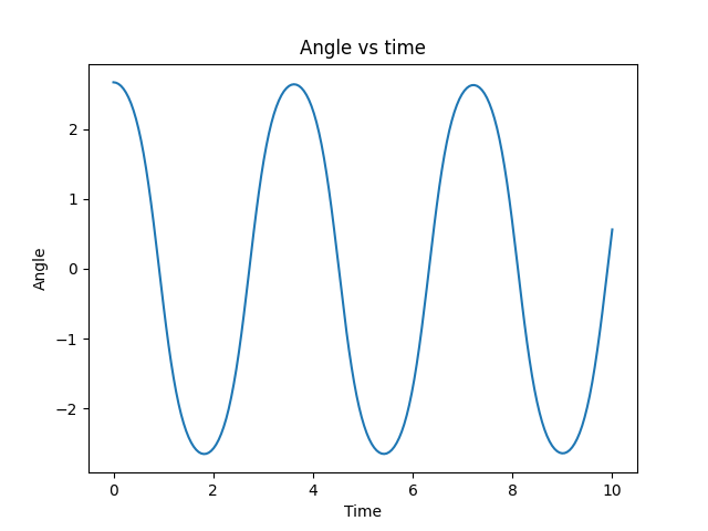
\[\mathbf{f}(z_1, z_2) = (z_2, - g\sin(z_1))\]Note that the function returns the change in position and the change in velocity. With that, a simple numerical ODE solver such as Euler’s method should do. I use the default settings in the ‘solve_ivp’ from Scipy. Then for a given initial condition (in this case \(0.85 \pi\) initial position and \(0\) initial velocity.) we can visualize the solution:
It looks a bit weird, and that is because it does not have any friction, it conserves the initial energy forever. We can visualize the evolution of the angle in time and we will see that it is indeed a perfect sinusoidal wave. With friction we expect a dumped oscillator.
Adding friction
Friction can be added to the equation of motion as a term that is proportional to the velocity. This is, the equation of motion becomes:
\[\ddot{\theta} = - g\sin(\theta) - c \dot{\theta}\]This makes the animations look more realistic, here I use a damping factor of 0.1.
Solving the pendulum equations.
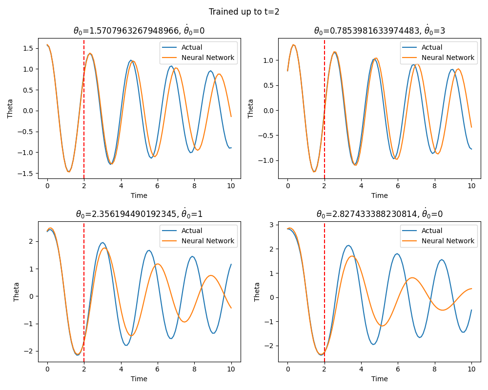
As I mentioned above, here I am going to take a data-driven approach. Nevertheless, using a naive neural network, even with a PINN like loss (using the second derivative as extra penalty) function does not work. It trivially interpolates the seen data, but it is not able to generalize to unseen \(t\), which is also sort of expected. There is an interesting paper around this: Neural Networks Fail to Learn Periodic Functions and How to Fix It, nevertheless their proposed solution also did not work for me. As an example:
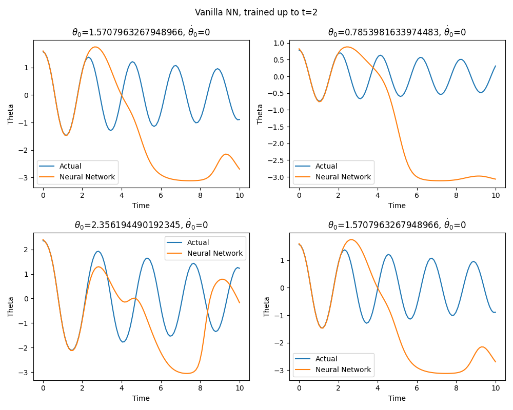
The title of each plot is the initial condition, blue is the simulated solution and orange is the neural network solution. It is clear that, beyond the training data, the neural network fails.
So, naive approaches will not work, and probably there is a lesson to be learned here about the extrapolating capabilities of neural networks. Anyway, now I dive into how to address this using a Koopman operator-like approach. Essentially this boils down to construct a basis where the system advances linearly. In this case, I use a simple autoencoder to approximate this basis. In what follows I essentially replicate the paper by Lusch et al. (reference 3).
As explained in the paper the pendulum has a continuous spectrum, meaning that has infinite possible frequencies. This implies that a simple linear model (which essentially describes a limited number of frequencies and/or decay/growth rates) will not be able to capture the full possible behaviors of the system. To address this, more flexibility is needed. What they propose is to use an auxiliary network to parameterize the eigenvalues of this linear model in a continuous fashion. In this way, we do not need infinite dimensional operator to approximate infinite frequencies.
Long story short, construct some latent space with an autoencoder such that we can find the next time step using a linear model in this latent space.
Complex numbers as rotation matrices, using Jordan canonical form to parameterize the eigenvalues.
A bit of background is needed to understand the next approach. In the paper they parameterize the eigenvalues directly, and, since we do not want to have to deal with complex types inside our neural network, a bit of math is needed. Complex eigenvalue pairs can be represented in a real block-diagonal matrix using the Jordan canonical form. This is because it is the same to multiply a two complex numbers as to multiply a vector by a 2x2 matrix:
\[(a + bi)(c + di) = (ac - bd) + (ad + bc)i\]and
\[\begin{bmatrix} a & -b \\ b & a \end{bmatrix} \begin{bmatrix} c \\ d \end{bmatrix} = \begin{bmatrix} ac - bd \\ ad + bc \end{bmatrix}.\]To specify a particular angle, we can use the polar coordinate form to see that (using angle sum and difference identities ):
\[(a + bi)(c + di) = r(\cos(\theta) + i\sin(\theta)) \cdot z(\cos(\phi) + i\sin(\phi)) = r z (\cos(\theta + \phi) + i\sin(\theta + \phi))\]Which for a magnitude of 1, this is equivalent to a rotation matrix (determinant 1) in 2D:
\[\begin{bmatrix} \cos(\theta) & -\sin(\theta) \\ \sin(\theta) & \cos(\theta) \end{bmatrix} \cdot \begin{bmatrix} \cos(\phi) \\ \sin(\phi) \end{bmatrix} = \begin{bmatrix} \cos(\theta + \phi) \\ \sin(\theta + \phi) \end{bmatrix}.\]This will be the kind of linear (“kind of” because \(\theta\) is parameterized by a non-linear function) that will advance the system in time. Here the expressive power of a neural net is constrained to fit a very particular form. Additionally, a magnitude is needed to specify dumped oscillators, this will also be given by the auxiliary network, essentially parameterizing a complex number in polar form.
Finally, we need to add the time displacement, so the Koopman operator (for a latent space of 2 dimensions) will look like:
\[\mathbf{K}(\theta, r, \Delta t) = r\begin{bmatrix} \cos(\theta \cdot \Delta t) & -\sin(\theta \cdot \Delta t) \\ \sin(\theta \cdot \Delta t) & \cos(\theta \cdot \Delta t) \end{bmatrix},\]Where \((\theta, r) = f_{\text{aux}}(z(t))\) and \(z(t)\) is the latent space representation of the system at time \(t\). Note that the latent space can be of any dimension, but care must be taken with the fact that rotation matrices work in 2D.
Network architecture, objective functions and training.
I simplify the objective function proposed by the paper by just taking an autoencoder reconstruction loss and a linear dynamics loss. The autoencoder reconstruction loss is simply the MSE of the reconstructed input without advancing it in time:
\[\mathcal{L}_{\text{AE}} = \frac{\sum_i ||x_t^i - f_{\text{dec}}(f_{\text{enc}}(x_t^i))||^2}{N}.\]The linear dynamic loss:
\[\mathcal{L}_{\text{dyn}} = \frac{\sum_i ||x_{\Delta t}^i - f_{\text{dec}}\bigl(\mathbf{K}(f_{\text{aux}}(f_{\text{enc}}(x_0^i)), \Delta t) \cdot f_{\text{enc}}(x_0^i)\bigr)||^2}{N}.\]Being \(\mathbf{K}\) the matrix that advances \(x_0\) (a vector of angle and velocity of the pendulum at time 0) to \(x_t\) in time. The training data, therefore, consists of tuples \((t, \theta_0, \dot{\theta}_0, \theta_t, \dot{\theta}_t)\). The network takes initial conditions and returns the position and velocity at time \(t\) and looks like:
Koopman_autoencoder(
  (encoder): encoder(
    (encoder): Sequential(
      (0): Linear(in_features=2, out_features=64, bias=True)
      (1): GELU(approximate='none')
      (2): Linear(in_features=64, out_features=64, bias=True)
      (3): GELU(approximate='none')
      (4): Linear(in_features=64, out_features=64, bias=True)
      (5): GELU(approximate='none')
      (6): Linear(in_features=64, out_features=2, bias=True)
    )
  )
  (decoder): decoder(
    (decoder): Sequential(
      (0): Linear(in_features=2, out_features=64, bias=True)
      (1): GELU(approximate='none')
      (2): Linear(in_features=64, out_features=64, bias=True)
      (3): GELU(approximate='none')
      (4): Linear(in_features=64, out_features=64, bias=True)
      (5): GELU(approximate='none')
      (6): Linear(in_features=64, out_features=2, bias=True)
    )
  )
  (K): K(
    (auxiliary_network): Sequential(
      (0): Linear(in_features=2, out_features=64, bias=True)
      (1): GELU(approximate='none')
      (2): Linear(in_features=64, out_features=64, bias=True)
      (3): GELU(approximate='none')
      (4): Linear(in_features=64, out_features=2, bias=True)
    )
  )
)
After training I get quite alright extrapolation (definitely superior to the naive approach) performance, not perfect, however:
Checking the latent space
Probably the most interesting plot here is the next one:
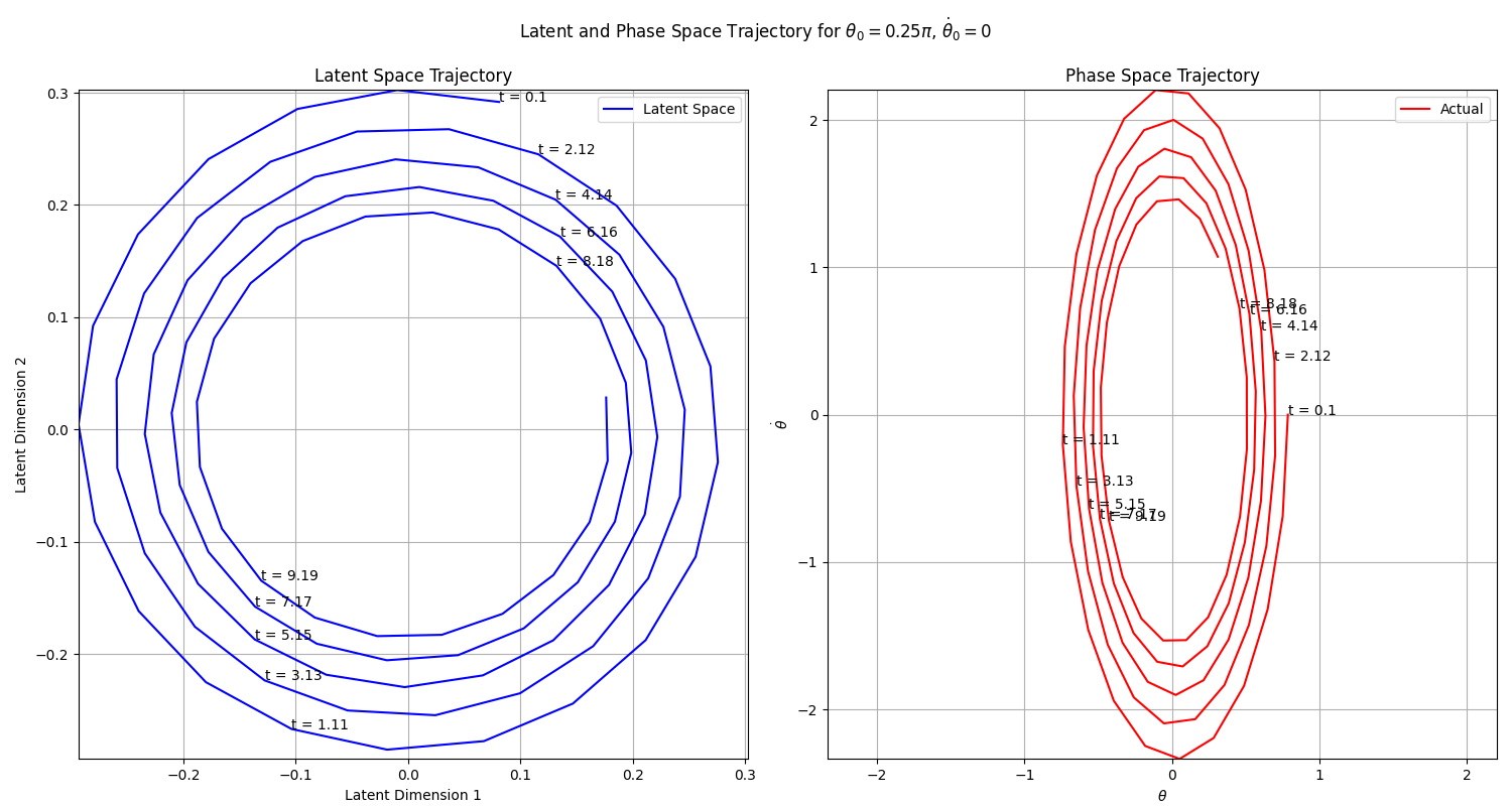
In phase space, the system describes an ellipse. This can be appreciated also above in the vector field plot. To be able to advance the system using a linear model, the coordinate system has to be transformed such that trajectories can be described by a circle (spiral circle in this case because of the friction). Going from an ellipse to a circle seems simple enough, particularly since the ellipse presents also this cycle behavior. It would be more interesting to check if this kind of approach could work with a system whose phase space is very far from cyclic.
In any case, it is quite satisfying to see that the autoencoder learns exactly the mapping that one would expect, very cool paper!
The code for making these figures and so on is available here.
-
See the first reference for the proof. ↩