All the code for this post can be found here!

From Optimal Separating Hyperplane to Support Vector Machines

Previously we already explained the basics of Optimal Separating Hyperplanes. There we considered the problem of optimally separating hyperplanes also with expansions of the input space, which allowed perfect separability of the classes. That extension was already in Support Vector Machines (SVMs) territory, but we did not consider the soft margin. Furthermore, there we used an off-the-shelf library for the QP problem. Here we slightly generalize the framework to that of the SVMs. The focus here, however, is on the optimization part of the problem, on the “technical” side. We will dive with quite a lot of detail into inequality constraint optimization theory for convex problems, with the SVM problem bieng just an illustration (a rather simple one) of the applicability of those algorithms.

In essence, SVM is a optimal separating hyperplane with two additions; first, the mapping of the input space to a high-dimensional feature space (e.g.,polynomial expansion of degree $d$). Second, soft margin classification, which allows non-perfect separability of the classes.

After solving for the primal and plugging in the solution, we have the following dual problem for the optimal separating hyperplane:

\[\begin{align*} \text{maximize}_{\alpha} \quad & \sum_{i=1}^n \alpha_i - \frac{1}{2} \sum_{i=1}^n \sum_{j=1}^n \alpha_i \alpha_j y_i y_j \mathbf{x}_i^\top \mathbf{x}_j \\ \text{subject to} \quad & \sum_{i=1}^n \alpha_i y_i = 0, \\ & \alpha_i \geq 0, \quad i = 1, \dots, n. \end{align*}\]

Generalizing this to the soft margin hyperplane is very simple, introducing a complexity parameter $C$:

\[\begin{align*} \text{maximize}_{\alpha} \quad & \sum_{i=1}^n \alpha_i - \frac{1}{2} \sum_{i=1}^n \sum_{j=1}^n \alpha_i \alpha_j y_i y_j \mathbf{x}_i^\top \mathbf{x}_j \\ \text{subject to} \quad & \sum_{i=1}^n \alpha_i y_i = 0, \\ & 0 \le \alpha_i \le C, \quad i = 1, \dots, n. \end{align*}\]

Intuitively, $C$ is an upper bound on the Lagrange multiplier associated with an observation. It limits the importance of the constraint of proper classification of the points. The higher $C$ the more importance it has to missclasify, with a very big $C$ we recover the hard-margin classifier because the “natural” Lagrange multipliers will be below $C$.

The combination of basis expansion with maximum margin separation is extremely interesting from the statistical learning perspective. The conceptual motivation for SVMs is a very rich topic. Rather than selecting a hypothesis by directly controlling model complexity through the number of parameters or network architecture, SVMs introduce an inductive bias based on margin maximization. The inductive step is taken by restricting attention to classifiers that achieve zero empirical risk on the training data (in the separable case), and among these, choosing the one that minimizes an upper bound on the probability of misclassification on unseen data. This shift, from fitting capacity to maximum margin, marks a fundamental departure from more traditional forms of inductive bias.

We will dive into the “conceptual” problem of SVMs in a future post.

For now, let’s dive into inequality constrained convex optimization. Note that an explanation of Newton’s method for equality constrained optimization is available here. We build from there.

Inequality constrained optimization

Often when looking into how SVM works, at some point a QP solver is invoked. We will code that explicitly. Here we illustrate two interior point methods and an ad-hoc algorithm for SVMs. In the first two points we loosely follow chapter 11 from [1].

log-barrier method

It is not immediately clear how one go about solving an inequality constrained minimization problem. Equality constrained minimization seems easier, we just have to make updates orthogonal to the constraint matrix. Perhaps the first thing that one can try is to add a penalty that goes to $\infty$ assuming we are minimizing (wlog).

The Log Barrier method is a rigorous approach in that direction.

Define the barrier functional:

\[\phi(x) = - \sum_{i=1}^m \log{(-f_i(x))}.\]

This function clearly goes to $\infty$ when $x \rightarrow 0$, and it is only defined for $f_i(x) < 0$. Hence, this is a perfect penalty to add to our objective function, transforming the inequality constrained optimization problem into an equality constrained optimization one. However, to not change the objective we want to optimize, we need to make the penalty very small when the parameters are feasible. To do that a constant “small” $t > 0$ is added.

The gradient and Hessian of $\phi(x)$ are very important:

\[\begin{align*} \nabla \phi(x) &= -\sum_{i=1}^m \frac{1}{f_i(x)} \, \nabla f_i(x) \\ \nabla^2 \phi(x) &= \sum_{i=1}^m \frac{1}{f_i(x)^2} \, \nabla f_i(x) \, \nabla f_i(x)^\top + \sum_{i=1}^m \frac{1}{f_i(x)} \, \nabla^2 f_i(x) \end{align*}\]

For the SVM case we have two inequality constraints $f^i_1(\alpha) = -\alpha_i \leq 0$ ($\alpha$ must be positive) and $f^i_2(\alpha) = \alpha_i - C \leq 0$ ($\alpha$ must be below $C$). In this case the barrier functional is (note that we are maximizing, so the first sign is changed to look for $-\infty$):

\[\phi(\alpha) = \sum_{i=1}^m \big( \log{(-f^i_1(x))} + \log{( - f^i_1(x))} \big) = \sum_{i=1}^m \big( \log{\alpha_i} + \log{(C - \alpha_i)} \big).\]

Hence, the new centralizer problem is:

\[\begin{align*} \text{maximize}_{\alpha} \quad & \sum_{i=1}^n \alpha_i - \frac{1}{2} \sum_{i=1}^n \sum_{j=1}^n \alpha_i \alpha_j y_i y_j \mathbf{x}_i^\top \mathbf{x}_j + t \sum_{i=1}^n \Big( \log \alpha_i + \log (C - \alpha_i) \Big) \\ \text{subject to} \quad & \sum_{i=1}^n \alpha_i y_i = 0, \end{align*}\]

Clearly, for each value of $t$ we have a different solution for this problem; we call them $\alpha^*(t)$. Now, one could choose a very small $t$ and just fit Newton’s method for equality constraints. However, this is unlikely to work well, because the Hessian is likely to vary very rapidly when the parameters of the inequality constraints are close to 0 (as per the Hessian definition above). In that case, the Lipschitz constant of the Hessian is huge, and we may need many iterations (to find a region where the gradient is already tiny) to reach the quadratically convergent phase of Newton’s method. Hence, the idea is to decrease $t$ “slowly” and initialize the Newton’s method in the previous solution, effectively having an outer loop decreasing $t$ and an inner loop solving the respective equality constrained problems starting at the solution of the previous iteration.

In any case, it is not completely obvious that this should yield the actual optimal for the original inequality constrained problem. Nevertheless, this is actually the case. In particular, for the general minimization case (assuming $f_0$ convex and differentiable, affine equality constraints ($h_i$) and convex inequality constraints ($f_i$)):

\[\lim_{t \rightarrow 0} f_0(x^*(t)) = f_0(x^*).\]

When $t$ is very small, then the objective value associated to the optimal parameters of the centralizer problem does indeed converge to the objective value of the optimal parameters in the original problem. To see this, note the following parallelism between the stationarity condition of the Lagrangian of the centralizer problem and the stationary condition of the original problem. For the centralizer problem:

\[\nabla f_0(x^*(t)) + t \nabla \phi (x^*(t)) + A^{\top}\nu^*(t) = 0,\]

for the original problem:

\[\nabla f_0(x^*) + \sum_{i=1}^m \lambda^*_i \nabla f_i(x^*) + A^{\top}\nu^* = 0.\]

Since $\nabla \phi(x) = -\sum_{i=1}^m \frac{1}{f_i(x)} \, \nabla f_i(x)$ then we have that we can define

\[\begin{equation} \lambda^*(t) = -\frac{t}{f_i(x^*(t))}, \label{eq:subst} \end{equation}\]

then the dual becomes (assuming $x^*(t)$ is feasible)

\[f_0(x^*) \geq g(\lambda^*(t), \nu^*(t)) = f_0(x^*(t)) + \sum_{i=1}^m \lambda_i^*(t) f_i(x^*(t)) + \nu^{*}(t)^\top (Ax^*(t) - b) = f_0(x^*(t)) - mt.\]

Hence, $x^*(t)$ is only $mt$ suboptimal so indeed the intuition is correct and we will recover the optimal solution. Note that, without strict convexity, $x^*$ might not be unique!

Finally, note that we do require always work with a feasible $x$. This is again not trivial; in fact, it requires an optimization step in itself (solving $Ax = b$ for $x \leq 0$ is as hard as an LP!). This boils down to solving:

\[\begin{aligned} \text{minimize}_{x, s} \quad & s \\ \text{subject to} \quad & Ax = b, \\ & f_i(x) \le s, \quad i = 1,\dots,n. \end{aligned}\]

Which is AGAIN an inequality constrained optimization problem. However, it suffices to solve this once with a “big” $t$.

The algorithm pieces for the general case

We derive now the Newton’s equations for the general case.

Phase I (finding a feasible initial point)

Construct the Lagrangian for a big $t$:

\[L(x, s, \nu) = s - t\sum_{i = 1}^m \log(s - f_i(x)) + \nu^{\top}(Ax -b).\]

Gradients and Hessians:

\[\begin{align*} \nabla_x L(x, s, \nu) &= \sum_{i=1}^m \frac{t}{s - f_i(x)} \nabla f_i(x) + A^\top \nu, \\ \nabla_s L(x, s, \nu) &= 1 - \sum_{i=1}^m \frac{t}{s - f_i(x)}, \\ \nabla_\nu L(x, s, \nu) &= Ax - b, \end{align*}\] \[\begin{align*} \nabla_x^2 L(x, s, \nu) &= \sum_{i=1}^m \left( \frac{t}{s - f_i(x)}\nabla^2 f_i(x) + \frac{t}{(s - f_i(x))^2} \nabla f_i(x) \nabla f_i(x)^\top \right), \\ \nabla_s^2 L(x, s, \nu) &= \sum_{i=1}^m \frac{t}{(s - f_i(x))^2}, \\ \nabla_{xs}^2 L(x, s, \nu) &= - \sum_{i=1}^m \frac{t}{(s - f_i(x))^2} \nabla f_i(x),\\ \nabla_{\nu x}^2 L(x, s, \nu) &= A, \\ \nabla_{\nu s}^2 L(x, s, \nu) &= 0, \\ \nabla_{\nu \nu}^2 L(x, s, \nu) &= 0. \end{align*}\]

Now, putting it all together:

\[\begin{bmatrix} \nabla_x^2 L & \nabla_{xs}^2 L & A^\top \\ (\nabla_{xs}^2 L)^\top & \nabla_s^2 L & 0 \\ A & 0 & 0 \end{bmatrix} \begin{bmatrix} \Delta x \\ \Delta s \\ \Delta \nu \end{bmatrix} = - \begin{bmatrix} \nabla_x L \\ \nabla_s L \\ \nabla_\nu L \end{bmatrix}\]

Centering step

\[L(x, \nu) = f_0(x) - t\sum_{i = 1}^m \log(-f_i(x)) + \nu^{\top}(Ax -b).\] \[\begin{bmatrix} \nabla^2 f_0(x) + t \nabla^2 \phi(x) & A^\top \\ A & 0 \end{bmatrix} \begin{bmatrix} \Delta x \\ \Delta \nu \end{bmatrix} = - \begin{bmatrix} \nabla f_0(x) + t \nabla \phi(x) + A^\top \nu \\ Ax - b \end{bmatrix}\]

However, since $x$ is feasible, we can focus on the simpler system (this simplification is not applied below, with no effect besides making the whole description and the code a bit more cumbersome):

\[\begin{bmatrix} \nabla^2 f_0(x) + t \nabla^2 \phi(x) & A^\top \\ A & 0 \end{bmatrix} \begin{bmatrix} \Delta x \\ \nu \end{bmatrix} = - \begin{bmatrix} \nabla f_0(x) + t \nabla \phi(x) \\ 0 \end{bmatrix}\]

log-barrier Method SVM algorithm

Now we’ve got everything we need. Bear in mind that we are optimizing the dual of the SVM, so we have a maximization problem! Furthermore, note that there are only 2 inequality constraints and 1 equality constraint acting in $\alpha$ as a vector.

First, let’s get the derivatives and Hessians for the Phase I and central path problems.

The Lagrangian for Phase I is:

\[L(\alpha, s, \nu) = s - t \sum_{i=1}^n \left( \log(s + \alpha_i) + \log(s + C - \alpha_i) \right) + \nu (\mathbf{y}^\top \alpha).\] \[\begin{align*} \nabla_\alpha L &= -t \left( \frac{1}{s + \alpha} - \frac{1}{s + C - \alpha} \right) + \nu \mathbf{y} \quad \text{Using elementwise division, } \nu \in \mathbb{R} \text{ (scalar)},\\ \nabla_s L &= 1 - t \sum_{i=1}^n \left( \frac{1}{s + \alpha_i} + \frac{1}{s + C - \alpha_i} \right), \\ \nabla_\nu L &= \mathbf{y}^\top \alpha. \end{align*}\]

Let $d_1 = \frac{1}{(s+\alpha)^2}$ and $d_2 = \frac{1}{(C + s -\alpha)^2}$ elementwise!

\[\begin{align*} \nabla_{\alpha \alpha}^2 L &= t \, \text{diag}(d_1 + d_2), \\ \nabla_{ss}^2 L &= t \sum_{i=1}^n (d_1 + d_2), \\ \nabla_{\alpha s}^2 L &= t (d_1 - d_2). \end{align*}\]

Finally:

\[\begin{bmatrix} t \, \text{diag}(d_1 + d_2) & t(d_1 - d_2) & \mathbf{y} \\ t(d_1 - d_2)^\top & t \sum (d_1 + d_2) & 0 \\ \mathbf{y}^\top & 0 & 0 \end{bmatrix} \begin{bmatrix} \Delta \alpha \\ \Delta s \\ \Delta \nu \end{bmatrix} = - \begin{bmatrix} \nabla_\alpha L \\ \nabla_s L \\ \mathbf{y}^\top \alpha \end{bmatrix}.\]

The Lagrangian for the Central Path problems is:

\[L(\alpha, \nu) = \mathbf{1}^\top \alpha - \frac{1}{2} \alpha^\top Q \alpha + t \sum_{i=1}^n \Big( \log \alpha_i + \log (C - \alpha_i) \Big) + \nu (\mathbf{y}^\top \alpha),\]

where $Q_{ij} = y_i y_j \mathbf{x}_i^\top \mathbf{x}_j$. Note the change of sign, the penalty goes negative because we are maximizing.

Again, gradients, Hessians, and Newton’s matrix (abusing a bit the elementwise operations…):

\[\begin{align*} \nabla_{\alpha} L &= \mathbf{1} - Q\alpha + t \left( \frac{1}{\alpha} - \frac{1}{C - \alpha} \right) + \nu \mathbf{y}, \\ \nabla_\nu L &= \mathbf{y}^\top \alpha, \end{align*}\]

Let $d_1 = \frac{1}{\alpha^2}$ and $d_2 = \frac{1}{(C -\alpha)^2}$ elementwise!

\[\begin{align*} \nabla_{\alpha \alpha}^2 L &= -Q - t \, \text{diag}(d_1 + d_2,) \\ \nabla_{\nu \alpha}^2 L &= \mathbf{y}^\top ,\\ \nabla_{\nu \nu}^2 L &= 0. \\ \end{align*}\]

And finally

\[\begin{bmatrix} -Q - t \, \text{diag}(d_1 + d_2) & \mathbf{y} \\ \mathbf{y}^\top & 0 \end{bmatrix} \begin{bmatrix} \Delta \alpha \\ \Delta \nu \end{bmatrix} = - \begin{bmatrix} \nabla_\alpha L \\ \nabla_\nu L \end{bmatrix}\]

Now all the math is ready, the algorithm then is:

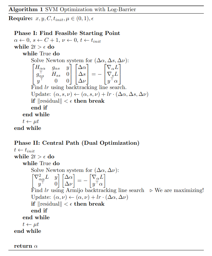
In the above demo we used RBF kernel for coolness purposes, but that has actually nothing to do with the optimization problem since it is literally just a different $Q$. In the code implementation and the above algorithm we are updating $\nu$. This is not necessary and is actually not part of the canonical log-barrier method which is strictly a primal algorithm. Here we are doing a primal-dual algorithm (because of $\nu$), even though this is not necessary since $x$ is guaranteed to be feasible.

Primal-Dual algorithm

The log-barrier method can be interpreted as solving a modified KKT system in each inner loop. A “continuous deformation” that indeed converges to the final canonical KKT system. In particular, again for the standard minimization problem:

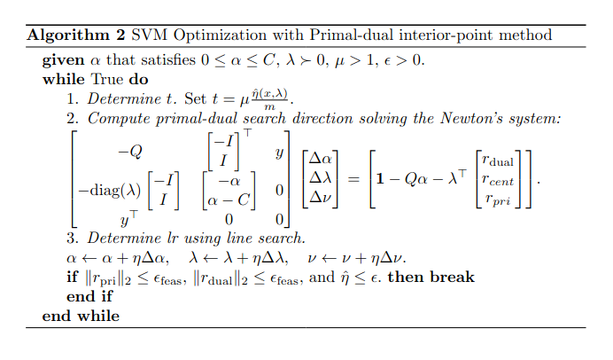
\[\begin{aligned} Ax &= b, \\ f_i(x) &\le 0, \quad i = 1,\dots,m, \\ \lambda &\ge 0, \\[6pt] \nabla f_0(x) + \sum_{i=1}^m \lambda_i \nabla f_i(x) + A^{T}\nu &= 0, \\[6pt] -\lambda_i f_i(x) &= t, \quad i = 1,\dots,m. \end{aligned}\]

The only difference is in the complementary slackness condition. In the log-barrier method $\lambda$ is eliminated via substitution (equation \ref{eq:subst}). The idea now is to directly focus on solving the modified KKT directly, explicitly optimizing $\lambda$. This greatly simplifies things. First, now we are allowed to work with not feasible values for primal and dual variables, hence; we skip Phase I altogether (which should make this already trivially twice as fast…). Convergence will ensure feasibility, but it is not a requirement at the start! (Which is why below the evolution of the objective function is not monotonically increasing.) Second, there is only one loop, $t$ is updated at the same time as $\lambda, x, \nu$.

Let’s check the theory again for the standard case and then we fill it in with the SVM problem specifics. The modified KKT equation to solve is:

\[\begin{bmatrix} \nabla^2 f_0(x) + \sum_{i=1}^m \lambda_i \nabla^2 f_i(x) & Df(x)^T & A^T \\ -\mathbf{diag}(\lambda)Df(x) & -\mathbf{diag}(f(x)) & 0 \\ A & 0 & 0 \end{bmatrix} \begin{bmatrix} \Delta x \\ \Delta \lambda \\ \Delta \nu \end{bmatrix} = - \begin{bmatrix} \nabla f_0(x) + Df(x)^{T}\lambda + A^{T}\nu \\ - \operatorname{diag}(\lambda)\, f(x) - t\mathbf{1} \\ Ax - b \end{bmatrix}\]

Define $\hat{\eta}(x, \lambda) = - \sum_{i=1}^m f_i(x)\lambda_i$.

\[\bigg\|\begin{bmatrix} \nabla f_0(x) + Df(x)^{T}\lambda + A^{T}\nu \\ - \operatorname{diag}(\lambda)\, f(x) - t\mathbf{1} \\ Ax - b \end{bmatrix}\bigg\|_2 = 0,\]

then $\hat{\eta}(x, \lambda) = mt$. If $\lambda, x, \nu$ satisfies the modified KKT, then $mt$ is the duality gap. Note that then $t = \frac{\hat{\eta}(x, \lambda)}{m}$. And here we have the idea for the algorithm, we are going to decrease the duality gap by decreasing $t$ (as before, using $\mu \in (0, 1)$) and at the same time forcing feasibility by the minimization of the residual. ¹

Now, turning back to SVMs.

Residuals:

\[\begin{align*} r_{\text{dual}} &= \mathbf{1} - Q \alpha - \lambda^{\top} \begin{bmatrix} -\mathbf{I} \\ \mathbf{I} \end{bmatrix} + \nu y \\ r_{\text{cent}} &= -\text{diag}(\lambda)\begin{bmatrix} -\alpha \\ \alpha - C \end{bmatrix} -t\mathbf{1} \quad \lambda \text{ is positive and the function values are negative (when feasible)}\\ r_{\text{pri}} &= \mathbf{y}^\top \alpha. \end{align*}\]

So the KKT matrix:

\[\begin{bmatrix} - Q & \begin{bmatrix}-I \\ I \end{bmatrix}^\top & y \\ -\text{diag}(\lambda) \begin{bmatrix}-I \\ I \end{bmatrix} & \text{diag}\begin{bmatrix} -\alpha \\ \alpha - C \end{bmatrix} & 0 \\ y^\top & 0 & 0 \end{bmatrix} \begin{bmatrix} \Delta \alpha \\ \Delta \lambda \\ \Delta \nu \end{bmatrix} = -\begin{bmatrix} \mathbf{1} - Q \alpha - \lambda^{\top} \begin{bmatrix} -\mathbf{I} \\ \mathbf{I} \end{bmatrix} + \nu y \\ -\text{diag}(\lambda)\begin{bmatrix} -\alpha \\ \alpha - C \end{bmatrix} -t\mathbf{1}\\ \mathbf{y}^\top \alpha \end{bmatrix}.\]

Note that, while in the log-barrier method we effectively inserted the inequality constraint in the Lagrangian and then continued (sort of) like in equaility constrained optimization, here we are NOT working on finding stationary points of any Lagrangian! Here everything follows from the residual vector. In other words, the modified KKT conditions here do not arise from the Lagrangian.

The line search must ensure that the $\lambda$ stays positive and the constraint functions negative. It also ensures that the norm of the residuals decreases sufficiently. From [1] §11.7:

One iteration of the primal-dual interior-point algorithm is the same as one step of the infeasible Newton method, applied to solving $\, r_t(x, \lambda, \nu) = 0$, but modified to ensure $\, \lambda > 0$ and $\, f(x) < 0$.

Finally, the algorithm:

Coding-wise, this felt much cleaner than the log-barrier method…

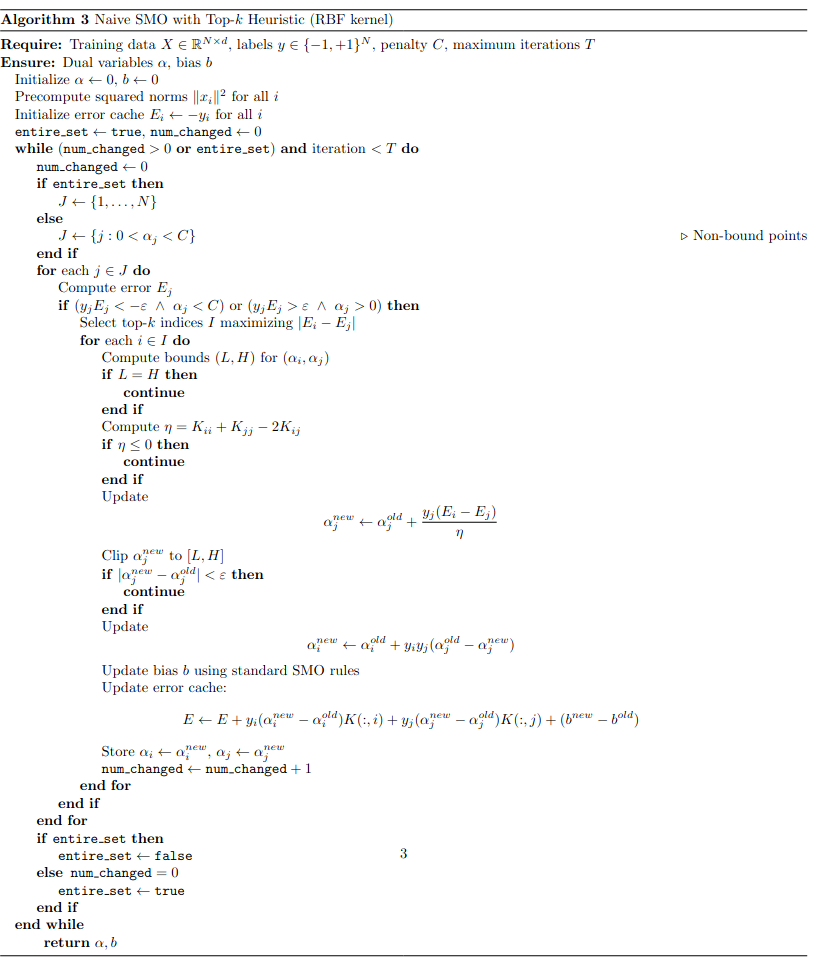
Sequential minimal optimization (SMO)

Derivation of the update equations

In 1998 Jonh C. Platt proposed an ad hoc algorithm for SVMs. The idea is basically a coordinate descent approach but with a catch. Again we are going to be dealing with the dual function. Optimizing one multiplier at a time is no possible because the linear equality constraint provides an identity that we have to respect. Imagine we are looking to optimize observation j:

\[- \sum_{i \neq j} y_i\alpha_i = \alpha_j y_j,\]

so we do not have any univariable direction of improvement that respects feasibility. So what now? Turns out that allowing for 2 degrees of freedom at each step actually allows increasing the dual function. The drawback is that then we have $N^2$ possible pairs to optimize, so a naive loop is absolutely terrible. Furthermore, in a real world scenario where SVMs generalize decently it is likely that $\alpha$ will be quite a sparse vector, so there may be updates that do not even increase the dual. In any case, heuristics are needed to solve this.

Let’s first derive the update rules, following [3] [4]. The aim is to exploit a closed form solution for

\[\begin{align*} \text{maximize}_{\alpha} \quad & \sum_{i=1}^n \alpha_i - \frac{1}{2} \sum_{i=1}^n \sum_{j=1}^n \alpha_i \alpha_j y_i y_j \mathbf{x}_i^\top \mathbf{x}_j \\ \text{subject to} \quad & \sum_{i=1}^n \alpha_i y_i = 0, \\ & 0 \le \alpha_i \le C, \quad i = 1, \dots, n. \end{align*}\]

if we let all $\alpha$ fixed but two, let’s call those two $\alpha_i$ and $\alpha_j$. Then we have that the pair-dual is:

\[D(\alpha_i, \alpha_j) = \alpha_i + \alpha_j +\sum_{k \neq i,j}^n \alpha_k - \frac{1}{2} \left[ \alpha_i^2 K_{ii} + \alpha_j^2 K_{jj} + 2 y_i y_j \alpha_i \alpha_j K_{ij} \right] - y_i \alpha_i \sum_{k \neq i,j}^n y_k \alpha_k K_{ik} - y_j \alpha_j \sum_{k \neq i,j}^n y_k \alpha_k K_{jk} - \frac{1}{2} \sum_{k \neq i,j}^n \sum_{m \neq i,j}^n y_k y_m \alpha_k \alpha_m K_{km}.\]

Where $K_{lm}$ is the inner product of $\phi(x_l)$ and $\phi(x_m)$ ($\phi(x)$ being a function that puts $x$ in another space, e.g., $n^{th}$ degree polynomial expansion). This is, a particular entry of the Kernel matrix.

Now, we have that, to respect the equality constraint:

\[y_i \alpha_i + y_j \alpha_j = - \sum_{k \neq i, j} y_k\alpha_k.\]

Multiplying both sides by $y_i$ (recall that $y$ is either $1$ or $-1$):

\[\alpha_i + y_iy_j \alpha_j = - y_i\sum_{k \neq i, j} y_k\alpha_k = \zeta,\]

hence,

\[\alpha_i = \zeta - y_iy_j \alpha_j .\]

We can plug this in and we get:

\[\begin{aligned} D(\alpha_j) &= \zeta + (1 - y_i y_j)\alpha_j - \frac{1}{2}\Big[ (\zeta - y_i y_j \alpha_j)^2 K_{ii} + \alpha_j^2 K_{jj} + 2 y_i y_j (\zeta - y_i y_j \alpha_j)\alpha_j K_{ij} \Big] \\ &\quad - y_i (\zeta - y_i y_j \alpha_j)\sum_{k\neq i,j} y_k \alpha_k K_{ik} - y_j \alpha_j \sum_{k\neq i,j} y_k \alpha_k K_{jk} + \text{const}. \end{aligned}\]

Rearranging the term within brackets we get:

\[\begin{aligned} (\zeta - y_i y_j \alpha_j)^2 K_{ii} &+ \alpha_j^2 K_{jj} + 2 y_i y_j (\zeta - y_i y_j \alpha_j)\alpha_j K_{ij} \\ &= \zeta^2 K_{ii} + 2 \zeta y_i y_j \alpha_j (K_{ij}-K_{ii}) + \alpha_j^2 (K_{ii}+K_{jj}-2K_{ij}). \end{aligned}\]

Rearranging the rest:

\[\begin{aligned} & \zeta + (1 - y_i y_j)\alpha_j - y_i (\zeta - y_i y_j \alpha_j)\sum_{k\neq i,j} y_k \alpha_k K_{ik} - y_j \alpha_j \sum_{k\neq i,j} y_k \alpha_k K_{jk} \\ &= \zeta + (1 - y_i y_j)\alpha_j - \zeta y_i \sum_{k\neq i,j} y_k \alpha_k K_{ik} + \alpha_j y_j \sum_{k\neq i,j} y_k \alpha_k K_{ik} - \alpha_j y_j \sum_{k\neq i,j} y_k \alpha_k K_{jk} \\ &= \zeta + (1 - y_i y_j)\alpha_j - \zeta y_i \sum_{k\neq i,j} y_k \alpha_k K_{ik} + \alpha_j y_j \sum_{k\neq i,j} y_k \alpha_k (K_{ik}-K_{jk}). \end{aligned}\]

Putting it together:

\[\begin{aligned} D(\alpha_j) &= - \frac{1}{2}\Big[\zeta^2 K_{ii} + 2 \zeta y_i y_j \alpha_j (K_{ij}-K_{ii}) + \alpha_j^2 (K_{ii}+K_{jj}-2K_{ij}) \Big] \\ &\quad - \zeta + (1 - y_i y_j)\alpha_j - \zeta y_i \sum_{k\neq i,j} y_k \alpha_k K_{ik} + \alpha_j y_j \sum_{k\neq i,j} y_k \alpha_k (K_{ik}-K_{jk}) + \text{const} \\ &= -\frac{1}{2}(K_{ii}+K_{jj}-2K_{ij})\alpha_j^2 +\alpha_j\Big[ (1-y_i y_j) -\zeta y_i y_j (K_{ij}-K_{ii}) + y_j \sum_{k\neq i,j} y_k \alpha_k (K_{ik}-K_{jk}) \Big] +\text{const}. \end{aligned}\]

Now we have a nice for for our scalar quadratic equation. However, we need to do a bit more work with the linear term. We have that:

\[y_j \sum_{k\neq i,j} y_k \alpha_k (K_{ik}-K_{jk}) = y_j \Bigg(\Big[u_i - b - \alpha_i y_i K_{ii} - \alpha_j y_j K_{ji} \Big] - \Big[u_j - b - \alpha_j y_j K_{jj} - \alpha_i y_i K_{ij} \Big]\Bigg),\]

where

\[u_i = \sum_{k=1}^N \alpha_k y_k K_{ki} + b,\]

this is, the prediction for the value $x_i$ in the hyperplane (note $w = \sum_{k=1}^N \alpha_k y_k \phi(x_k)$). Now, let $E_k = u_k - y_k$ be the error of the prediction. Substituting $\zeta$ back:

\[\begin{aligned} & (1-y_i y_j) -\zeta y_i y_j (K_{ij}-K_{ii}) + y_j \Bigg(\Big[u_i - b - \alpha_i y_i K_{ii} - \alpha_j y_j K_{ji} \Big] - \Big[u_j - b - \alpha_j y_j K_{jj} - \alpha_i y_i K_{ij} \Big]\Bigg) \\ &= (1-y_i y_j) + ( \alpha_iy_i y_j + \alpha_j) (K_{ii} - K_{ij}) + \Bigg( y_j(u_i - u_j) + \alpha_j K_{jj} - \alpha_i y_i y_j K_{ii} + \alpha_i y_j y_i K_{ji} - \alpha_j K_{ji}\Bigg) \\ & = (1-y_i y_j) + ( \alpha_i y_i y_j)(K_{ii} - K_{ij} - K_{ii} + K_{ji}) + (\alpha_j)(K_{ii} - K_{ij} + K_{jj} - K_{ji}) + y_j(u_i - u_j) \\ & = (1-y_i y_j) + \alpha_j(K_{ii} - 2K_{ij} + K_{jj}) + y_j(u_i - u_j).\\ \end{aligned}\]

And finally, since $E_i - E_j = u_i - y_i - u_j + y_j$:

\[\begin{aligned} &\alpha_j(K_{ii} - 2K_{ij} + K_{jj}) + y_j(E_i - E_j) \\ &= \alpha_j(K_{ii} - 2K_{ij} + K_{jj}) + y_ju_i - y_j y_i - y_j u_j + 1 \\ &= \alpha_j(K_{ii} - 2K_{ij} + K_{jj}) + (1-y_i y_j) + y_j(u_i - u_j). \end{aligned}\]

Hence we are ready to get the analytical solution:

\[\begin{aligned} D(\alpha_j) = -\frac{1}{2}(K_{ii}+K_{jj}-2K_{ij})\alpha_j^2 +\alpha_j\Big[ \alpha_j^{old}(K_{ii} - 2K_{ij} + K_{jj}) + y_j(E_i - E_j) \Big] +\text{const}. \end{aligned}\]

Importantly, note that $\alpha_j^{old}$ inside the brackets is a given value. Taking the derivative and equating to 0 we arrive at the solution:

\[\begin{equation} \alpha_j^{new} = \alpha_j^{old} + \frac{y_j(E_i - E_j)}{(K_{ii}+K_{jj}-2K_{ij})}, \quad \alpha_i^{new}= \zeta - y_jy_i \alpha_j^{new} = \alpha_i^{old} + y_i y_j(\alpha_j^{old} - \alpha_j^{new}). \label{eq:updateSMO} \end{equation}\]

The second equation follows from the fact that $y_jy_i\alpha_j^{old} + \alpha_i^{old} = \zeta$ since this is respected throughout.

Great! We’ve got a solution. Nevertheless, we still need to enforce the “box” constraints. There are two cases, either $y_iy_j$ is $1$ or $-1$. If it is $1$ then

\[\alpha_j + \alpha_i = \zeta.\]

Since $\alpha$ cannot be higher than $C$ or below 0. We have that if $\zeta < C$ the minimum for $\alpha_j$ is 0 and the maximum $\zeta$. On the other case, if $\zeta \geq C$ then the minimum is $\zeta - C$ (which implies $\alpha_i = C$ which is the upper limit) and the maximum is $C$. Hence the lower bound for $y_iy_j = 1$ is $\text{max}(0, \zeta - C)$ and the upper bound $\text{min}(\zeta, C)$. Reasoning in the same way for $y_iy_j = -1$ we have that the lower bound is $\text{max}(0, -\zeta)$ and the upper bound $\text{min}(C - \zeta, C)$. Those bounds have to be respected acting like a clip on the update, they ensure that the $\alpha$ remains feasible (e.g., think of projected gradient descent).

Finally, the updates in:

\[\begin{aligned} w^{new} &= \sum_{n \neq i, j} y_n \alpha^{old}_n x_n + y_j \alpha_j^{new}x_j + y_i \alpha_i^{new}x_i\\ &= w^{old} + y_j \alpha_j^{new}x_j - y_j \alpha_j^{old}x_j + y_i \alpha_i^{new}x_i - y_i \alpha_i^{old}x_i\\ &= w^{old} + y_j \triangle \alpha_jx_j + y_i \triangle \alpha_ix_i\\ \end{aligned}\]

And for $b$ we have two cases, if $\alpha_i$ or $\alpha_j$ are not at the bounds (note that in that case we have a support vector for at least one of the two), and hence, the error is 0. In that case we look for the $b$ that forces $u_k = y_k$. Suppose that $\alpha_i$ is not saturated, then:

\[b_i = y_i - w^{new}\phi(x_k) = \sum_{n=1}^N y_n \alpha^{new}_n K_{ni},\]

the same applies for $b_j$. If neither is saturated, either works. If both are saturated (non-support vectors or just wrongly classified), we take the average. The above formulation is intuitive but slow; in practice, it is better to use:

\[\begin{aligned} b_1 &= b^{old} - E^{old}_i - y_i(\alpha_i^{new} - \alpha_i^{old})K_{ii} - y_j(\alpha_j^{new} - \alpha_j^{old})K_{ij} \\ b_2 &= b^{old} - E^{old}_j - y_i(\alpha_i^{new} - \alpha_i^{old})K_{ij} - y_j(\alpha_j^{new} - \alpha_j^{old})K_{jj}. \end{aligned}\]

Which arises from (assuming $E_k^{new} = 0$):

\[\begin{aligned} & E_k^{new} - E_k^{old} = \sum_{n=1}^N y_n \alpha^{new}_n K_{ni} +b^{new}- \sum_{n=1}^N y_n \alpha^{old}_n K_{ni} - b^{old} \quad \text{focusing only on the terms that change}\\ & = y_i(\alpha_i^{new} - \alpha_i^{old})K_{ij} - y_j(\alpha_j^{new} - \alpha_j^{old})K_{jj} b^{new} - b^{old}. \\ \end{aligned}\]

Pair selection heuristics

As mentioned, a naive implementation has $N^2$ pairs to optimize. However, SMO uses heuristics to reduce the candidates. First, we have to ensure that at least one of the multipliers is violating KKT conditions. Second, the support vectors (non-saturated Lagrange multipliers) are the most likely to play a big role. The first heuristic, then, is loop over all the dataset and update the multipliers that violate KKT conditions, then loop only over the support vectors (several times if needed) until all support vectors comply with KKT conditions. Then the process is repeated, to make sure “no more” updates are possible. When no updates are made, the algorithm stops.

The second heuristic is to select the second multiplier once the first is selected. In the implementation for this post, we tried to use the argmax of the denominator of the update of $\alpha_j$ to select just the best step for each $\alpha_j$. While it worked ok-ish, it did not converge very close to the sklearn implementation of the SVM. Using all indices seemed to work perfect but is very wasteful. Taking just the top 50 seemed like an ok compromise so in this implementation we do 50 updates for each $\alpha_j$ focusing on the top $\alpha_i$ that are more likely to yield a change. Another option could be to compute the denominator, but this implies computing the whole kernel matrix. In any case, this likley is very far away from actual top performing implenentations of the algorithm, but that is beyond the post.

One particularly interesting bit of the SMO implementation is that, since the error at the beginning is known ($y$, since $w = 0$ and $b = 0$) and we update just a couple of multipliers at a time, we do not need to recompute all the errors but change the errors associated with the multipliers that we updated. This is very important.

Putting all together

The algorithm is relatively simple without the heuristics (essentially a “coupled” coordinate descent). In the code it looks something like follows:

In the optimization process one can tell the difference from the “global” Newton’s method step.

SVM in MNIST: Telling a 5 from a 3

An important thing to note is that, when selecting the support vectors to infer $b$ (for support vectors prediction matches the label exactly), we have to allow for some numerical room. This is, the filter has to be something like $0 - \epsilon < \alpha < C +\epsilon$. Finally, after all this, we can contemplate how the default SVM implementation obliterates our algorithms! This is obviously expected since sklearn SVM optimization process is based on libsvm which offers a highly optimized SMO algorithm. For some reason the gamma parameter in sklearn-SVM behaves differently than in my implementation. In any case, here are the results for 1232 training examples in 256 dimensions.

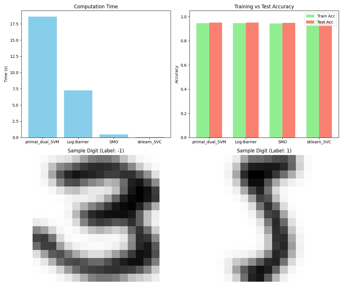
Quite cool that the algorithms are somewhat decent, taking into account this was pure numpy!

References

These notes are a personal synthesis and extensions based on lectures from Mastermath (NL) Continuous Optimization Course 2025 along with standard references (below). Any errors are my own.

Boyd, S., & Vandenberghe, L.
Convex Optimization
Vapnik, V. N.
The Nature of Statistical Learning Theory
HMC resource: SMO
John C. Platt A fast algorithm for Training SVM

Footnotes

That intuition is not complete for me... I am struggling to see this, the key is in the definition of the surrogate dual gap.

Steepest descent: A geometrical take from gradient descent to Newton's method.

Blog Archive

Archive of all previous blog posts