Steepest descent: A geometrical take from gradient descent to Newton's method.

Gradient descent with exact line search: convergence analysis

A key element in understanding gradient descent is its relationship with the condition number of the Hessian of the function we are minimizing. This will give an interesting framework to understand Newton’s method advantages. Let’s follow §9.3.1 from [1]. The idea here is to relate how many iterations we need to reach the optimum using gradient descent to the condition number of the Hessian.

The gradient descent algorithm with exact line search:

Algorithm: Gradient descent with exact line search

Given x0 in R^n, tolerance epsilon > 0

for k = 0, 1, 2, ...:
    g_k = grad f(x_k)
    if ||g_k|| <= epsilon:
        return x_k
    alpha_k = argmin_{alpha > 0} f(x_k - alpha*g_k)
    x_{k+1} = x_k - alpha_k * g_k

Note that this involves solving:

\[\alpha_k = \arg\min_{\alpha > 0} f(x_k - \alpha g_k),\]

which may or may not be difficult. For simplicity, let us assume that the exact optimal step is available.

Let $f(x): \mathbb{R^n} \rightarrow \mathbb{R}$ be a twice differentiable and strongly convex quadratic function (we relax this later).

In what follows we first derive a lower bound on the norm of the gradient and then an upper bound on the distance to the objective value after one iteration of the algorithm. The idea is to provide an upper bound on the distance to the optimal value as a function of the previous step.

Consider the second order Taylor approximation to $f$ around $x$ with Lagrange remainder:

\[f(y) = f(x) + \nabla f(x)^{\top}(y-x) + \frac{1}{2} (y-x)^{\top}\nabla ^2 f(z) (y - x),\]

for some $z = \theta x + (1-\theta) y \quad $ with $\theta \in [0, 1]$. Since $f$ is an strictly convex function we have that the second derivative must be positive definite ¹. Now, we want to find a lower and upper bound of $\frac{1}{2} (y-x)^{\top}\nabla ^2 f(z) (y - x)$. By considering the smallest eigenvalue $\nu_{min}$ of $\nabla ^2 f(z)$ ² we obtain a lower bound:

\[\begin{equation} f(y) \geq f(x) + \nabla f(x)^{\top}(y-x) + \frac{1}{2} \nu_{min}\|y - x\|^2_2. \label{eq:lowb} \end{equation}\]

From here, we can derive a lower bound on the difference to the optimal function value. Looking for the $\bar{y}$ that minimizies the r.h.s. of equation \ref{eq:lowb}. Equating the first derivative w.r.t $y$ to $0$:

\[\nabla f(x) + \nu_{min}(y-x) = 0,\]

then,

\[\bar{y} = x - \frac{\nabla f(x)}{\nu_{min}}.\]

Hence, plugging in, we have

\[\begin{align*} f(x) &+ \nabla f(x)^{\top}(y - x) + \frac{1}{2}\nu_{\min}\|y - x\|_2^2 \\ &\ge f(x) + \nabla f(x)^{\top}\!\left(-\frac{\nabla f(x)}{\nu_{\min}}\right) + \frac{1}{2}\nu_{\min} \|\frac{\nabla f(x)}{\nu_{\min}}\|_2^2 \\ &= f(x) - \frac{1}{\nu_{\min}}\|\nabla f(x)\|_2^2 + \frac{1}{2\nu_{\min}}\|\nabla f(x)\|_2^2 \\ &= f(x) - \frac{1}{2\nu_{\min}}\|\nabla f(x)\|_2^2 . \end{align*}\]

Finally, since the above holds for any $y$, we have that

\[\begin{equation} 2\nu_{\min}(-p^* + f(x)) \leq \|\nabla f(x)\|_2^2 \label{eq:lowbound_g} \end{equation}\]

Now for the upper bound:

\[\begin{equation} f(y) \leq f(x) + \nabla f(x)^{\top}(y-x) + \frac{1}{2} \nu_{max}\|y - x\|^2_2. \label{eq:uppb} \end{equation}\]

Let’s plug in the line search step in the above equation \eqref{eq:uppb} :

\[\begin{aligned} f(x - \alpha\nabla f(x)) &\leq f(x) + \nabla f(x)^{\top}\big((x - \alpha\nabla f(x)) - x\big) + \tfrac{1}{2}\nu_{\max}\|(x - \alpha\nabla f(x)) - x\|_2^2 \\ &= f(x) + \nabla f(x)^{\top}\big(-\alpha\nabla f(x)\big) + \tfrac{1}{2}\nu_{\max}\|(\alpha\nabla f(x))\|_2^2 \\ &= f(x) - \alpha\|\nabla f(x)\|^2_2 + \tfrac{\alpha^2}{2}\nu_{\max}\|\nabla f(x)\|_2^2. \end{aligned} \\\]

Now, minimizing over $\alpha$ (is a simple quadratic equation):

\[-\|\nabla f(x)\|^2_2 + \alpha\nu_{\max}\|\nabla f(x)\|_2^2 = 0\]

so the optimal $\alpha$:

\[\alpha = \frac{\|\nabla f(x)\|^2_2}{\nu_{\max}\|(\nabla f(x))\|_2^2} = \frac{1}{\nu_{\max}}.\]

Plugging in:

\[\begin{aligned} f(x - \alpha\nabla f(x)) & \leq f(x) - \frac{1}{\nu_{\max}}\|\nabla f(x)\|^2_2 + \frac{1}{2\nu_{\max}^2}\nu_{\max}\|\nabla f(x)\|_2^2 \\ &= f(x) - \frac{1}{\nu_{\max}}\|\nabla f(x)\|^2_2 + \frac{1}{2\nu_{\max}}\|\nabla f(x)\|_2^2 \\ &= f(x) - \frac{1}{2\nu_{\max}}\|\nabla f(x)\|^2_2. \end{aligned} \\\]

Substracting the optimal value $p^*$ and using equation \ref{eq:lowbound_g}:

\[\begin{aligned} f(x - \alpha \nabla f(x)) - p^* \leq f(x) - p^* - \frac{1}{2\nu_{\max}}\|\nabla f(x)\|^2_2 \leq f(x) - p^* - \frac{\nu_{\min}}{\nu_{\max}}(-p^* + f(x)) = (1 - \frac{\nu_{\min}}{\nu_{\max}})(f(x) - p^*) \end{aligned} \\\]

We are almost there. Appartenly if $\frac{\nu_{\min}}{\nu_{\max}} = 0$ is possible that we make no progress towards the optimum, since the value of the function after applying the optimal step may be the same. Let’s look closer:

Let

\[\begin{aligned} x_{k+1} := x_k - \alpha_k \nabla f(x_k),\\ \rho := 1 - \frac{\nu_{\min}}{\nu_{\max}}. \end{aligned} \\\]

Then, since $f(x_{k+1}) - p^* \leq \rho \bigl(f(x_k) - p^*\bigr)$, we have that

\[f(x_{k+2}) - p^* \leq \rho \bigl(f(x_{k+1}) - p^*\bigr) \leq \rho^2 \bigl(f(x_k) - p^*\bigr),\]

So, we have found a way of constructing an upper bound for any iteration in the algorithm based on the initial difference and the the smallest and biggest eigenvalue of the Hessian:

\[f(x_{k}) - p^* \leq \rho^k \bigl(f(x_0) - p^*\bigr).\]

Solving for $k$, we can make an explicit formula for the maximum number of iterations required to reach a particular loss. In particular, let $\epsilon$ be the desired suboptimality, we have that $f(x_{k}) - p^* \leq \epsilon$ if:

\[\begin{aligned} \rho^n = \frac{\epsilon}{\bigl(f(x_0) - p^*\bigr)}; \\ \log(\rho)n = \log(\frac{\epsilon}{\bigl(f(x_0) - p^*\bigr)}); \\ n = \frac{\log(\frac{\epsilon}{\bigl(f(x_0) - p^*\bigr)})}{\log(\rho)};\\ n = \frac{\log(\frac{\bigl(f(x_0) - p^*\bigr)}{\epsilon})}{\log(\frac{1}{\rho})} \\ \end{aligned}\]

Looking closer at the denominator we see that, if the condition number of the Hessian is big, $\rho$ approaches 1 and hence the denominator approaches 0, increasing the number of iterations required!

A note for arbitrary convex functions

Above, treating the quadratic case allowed to make intuitive use of the maximum and minimum eigenvalue. However, in general, this is not possible since the Hessian will be a function of $x$. Nevertheless, the above reasoning holds when changing the maximum and minimum eigenvalue by $M$ and $m$ respectively:

\[\nabla^2 f(x) - m I \in \mathbb{S}^n_+, \qquad M I - \nabla^2 f(x) \in \mathbb{S}^n_+ \quad \forall x \in Q.\]

For some set $Q$ being the domain of $f$, e.g. $\mathbb{R}^n$. $\mathbb{S}^n_+$ is the set of PSD matrices.

Steepest descent

Gradient descent is a particular instance of a more general framework. Let us now consider steepest descent, we will follow §9.4 from [1].

Again, we start with a Taylor approxmation, in this case, a first order one:

\[f(x + v) \approx f(x) + \nabla f(x)^{\top}(v).\]

The idea is now to minimize this approximation with respect to $v$, but with a constraint on the norm of $v$. The “normalized” steepest descent direction is defined then as:

\[\triangle x_{nsd} = \text{argmin}\{\nabla f(x)^\top v \: |\: \|v\| \leq 1 \},\]

for some norm. Selecting this norm is the key here.

We can also look at the “unnormalized” steepest descent direction:

\[\triangle x_{sd} = \|\nabla f(x)\|_*\triangle x_{nsd}.\]

We have that:

\[\|\nabla f(x)\|_* = \text{sup}\{\nabla f(x)^\top z \: : \|z\| \leq 1\}\]

i.e. what is the maximum directional derivative of $f$ at $x$ over all directions with unit norm? Following that line of thought we must have that:

\[\nabla f(x)^\top \triangle x_{nsd} = -\|\nabla f(x)\|_*.\]

Why? Because $ \triangle x_{nsd}$ is trying to find the direction with unit norm that minimizes the directional derivative. So, evaluating that directional derivative is exactly the definition of the dual norm up to a sign.

Euclidean norm: Gradient Descent

For the euclidean norm we have that, since we need a vector whose angle is 0 with the gradient but still unit norm,

\[\triangle x_{nsd} = -\frac{\nabla f(x)}{\|\nabla f(x)\|_2},\]

and hence,

\[\triangle x_{sd} = \|\nabla f(x)\|_*\triangle x_{nsd} = -{\|\nabla f(x)\|_2}\frac{\nabla f(x)}{\|\nabla f(x)\|_2} = -\nabla f(x).\]

Quadratic norm: Newton’s Method

The description above was intended to motivate Newton’s method advantage over gradient descent. In particular, the problem of gradient descent with high condition numbers of the Hessian even for simple quadratic equations.

Turns out that we can propose a change of basis where this problem dissapears! In fact, for quadratic equations we will need just one iteration. While this is somewhat obvious when treating Newton’s method as a root finding agorithm for a second degree Taylor approximation to the function, that interpretation does not illustrate the interesting geometry that is going on “behind” it.

So, let’s consider the quadratic norm to see how to get rid of the problematic condition number:

\[\|z\|_P = (z^\top P z)^{0.5} = \|P^{0.5}z\|_2,\]

where $P \in \mathbb{S}_{++}$ (a positive definite matrix). Let us then consider

\[\triangle x_{nsd} = \text{argmin}\{\nabla f(x)^\top v \: |\: \|v\|_P \leq 1 \}.\]

We need to solve this inequality constrained optimization problem. Here we solve it in a simple way, but there are other ways³:

\[\begin{aligned} \triangle x_{nsd} &= \text{argmin}\{\nabla f(x)^\top v \: |\: \|v\|_P \leq 1 \}, \\ &= \text{argmin}\{\nabla f(x)^\top v \: |\: v^tPv = 1 \}, \quad \text{since is a linear objective function, constraint must be saturated} \\ &= \text{argmin}\{\nabla f(x)^\top v \: |\: (P^{0.5}v)^\top(P^{0.5}v) = 1 \}, \\ &= P^{-0.5}\text{argmin}\{\nabla f(x)^\top P^{-0.5}u \: |\: u^\top u = 1 \}, \quad v = P^{-0.5}u \\ &= P^{-0.5}\text{argmin}\{ (P^{-0.5}\nabla f(x))^\top u \: |\: \| u \|_2= 1 \} \\ &= \frac{P^{-1}\nabla f(x)}{\| P^{-0.5}\nabla f(x) \|_2}.\\ \end{aligned}\]

And then \(\triangle x_{sd} = P^{-1}\nabla f\).

Change of basis interpretation

Let $\bar{x} = Ax$ and $\bar{f}(\bar{x}) = f(A^{-1}\bar{x})$ and let $A \in \mathbb{S}_{++}^n$. Essentially, $\bar{f}$ is a function that describes the same level sets in another basis:

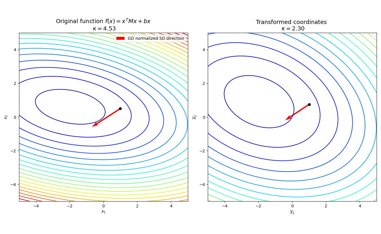
Illustration of a coordinate transformation: the left plot shows the original function, and the right plot shows the function on a different basis. The quadratic norm allows to pursue gradient descent for the same function on a different basis. In particular the linear transformation consist of an stretch of the vertical axis. Importantly, in this basis the condition number of the Hessian has improved.

Consider the derivative:

\[\nabla \bar{f}(\bar{x}) = A^{-1}\nabla f(A^{-1}\bar{x}) = A^{-1}\nabla f(x).\]

Now, mapping back to the original space, the search direction is:

\[v = A^{-2}\nabla f(x)\]

So, if we let $A = P^{0.5}$ then note that this has the same form as the normalized Steepest Descent direction for the quadratic norm. This shows that Steepest Descent with a quadratic norm is just gradient descent on a different basis ⁴ !

Newton’s Method algorithm

We now have all the pieces (it was more difficult than I expected…)!

Let $A = (\nabla^2 f(x))^{0.5}$. Then, $\nabla^2 \bar{f}(\bar{x}) = I$. The condition number is 1.

And that’s it, Newton’s method is a gradient descent method with change of basis that aliviates the condition number of the Hessian.

Algorithm: Newton's method

Given x0 in R^n, tolerance epsilon > 0

for k = 0, 1, 2, ...:
  Calculate Newton's step and decrement:
    v = -h_k(x)^{-1} g_k(x)
    lambda = g_k(x)^T h_k(x)^{-1} g_k(x)
  If lambda < epsilon:
    Quit
  Line search:
    Get alpha_k
  Update:
  x_k = x_{k-1} + alpha_k v

Convergence analysis for Newton’s method

This is going to be a digestion of §9.5.3 from [1], hopefully bringing us some intuition. Alright, recall that for quadratic functions Newton’s method is trivial, and in fact, those can be solved analytically. So here we will focus on arbitrary strongly convex and differentiable functions. Additionally we are going to assume:

\[\|\nabla^2 f(x) - \nabla^2 f(y) \|_2 \leq L\|x-y\|_2,\]

i.e. the Hessian is Lipschitz continuous. Essentially, $L$ will measure how good is the second order Taylor approximation for $f$.

The idea is to show that if we start close enough to the optimum $x^*$ then Newton’s method will converge quadratically. In this case we consider iterates of Newton’s method with unit stepsize (“pure Newton’s step”).

Let $\triangle_{nt} = -(\nabla^2 f(x))^{-1} \nabla f(x)$:

\[\begin{aligned} \|\nabla f(x_k + \triangle_{nt}^k)\|_2 = \|\nabla f(x_{k+1})\|_2 &= \| \nabla f(x_k + \triangle_{nt}^k) - \nabla f(x_k) + \nabla^2 f(x_k) (\nabla^2 f(x))^{-1} \nabla f(x)\|_2 \\ &= \| \nabla f(x_k + \triangle_{nt}^k) - \nabla f(x_k) - \nabla^2 f(x_k) \triangle_{nt}^k\|_2 \\ &= \| \int_0^1 \big( \nabla^2 f(x_k + t\triangle_{nt}^k) - \nabla^2 f(x_k) \big) dt \triangle_{nt}^k\|_2 \quad \text{(Fundamental theorem of calculus)} \\ &\leq \int_0^1 \| \big( \nabla^2 f(x_k + t\triangle_{nt}^k) - \nabla^2 f(x_k) \big) \triangle_{nt}^k\|_2dt \quad \text{(Triangle inequality)} \\ &\leq \int_0^1 \| \big( \nabla^2 f(x_k + t\triangle_{nt}^k) - \nabla^2 f(x_k) \big)\|_2\|\triangle_{nt}^k\|_2dt \quad \text{(Cauchy–Schwarz inequality)} \\ &\leq \int_0^1 L(t \|\triangle_{nt}^k \|_2 ) \|\triangle_{nt}^k \|_2 dt \quad \text{(Lipschitz continuity definition)} \\ &= \frac{L}{2}\|-(\nabla^2 f(x))^{-1} \nabla f(x)\|^2_2 \\ &\leq \frac{L}{2}\| m^{-1}\nabla f(x_k)\|^2_2 \quad \text{(Effect of the Hessian is bounded below by smallest eigenvalue possible in the domain)} \\ &= \frac{L}{2m^2}\| \nabla f(x_k)\|^2_2.\\ \end{aligned}\]

So, the norm of the gradient at $k+1$ is bounded above by some value proportional to the gradient at the $k$. We have that ⁵ \(f(x) - x^* \leq \frac{1}{2m} \| \nabla f(x)\|_2^2\) and that \(\frac{L}{2m^2} \|\nabla f(x_{k+1})\|_2 \leq \big( \frac{L}{2m^2}\| \nabla f(x_k)\|_2 \big)^2\) so:

\[\begin{aligned} f(x) - x^* &\leq \frac{1}{2m} \| \nabla f(x_k)\|_2^2 \\ &= \frac{2m^3}{L^2} \big(\frac{L}{2m^2}\| \nabla f(x_k)\|_2 \big)^2 \\ &\leq \frac{2m^3}{L^2} \big(\frac{L}{2m^2}\| \nabla f(x_{k-1})\|_2 \big)^4 \\ &\leq \cdots \\ &\leq \frac{2m^3}{L^2} \big(\frac{L}{2m^2}\| \nabla f(x_{0})\|_2 \big)^{2^{k + 1}} \\ \end{aligned}\]

So, if $| \nabla f(x_{0})|_2 < \frac{2m^2}{L}$ then covergence is extremely fast! Much faster than gradient descent. However, if we are far away from the optimum the algorithm could be very slow or diverge. In that case, line search is essential.

Importantly, note that the notion of distance depends on $L$ and $m$. In particular, note that if $L$ is huge, the gradient must be very small in order to enter the quadratic convergence regime! The more stable the Hessian is, the better. Intuitively, lower $L$ implies that the function resembles a quadratic function and hence the second order Taylor approximaton is better. This is particularly relevant for log-barrier methods but we will not dive into that here.

Some comments on equality constrained optimization

Let’s consider the following minimization problem:

\[\begin{aligned} \text{minimize}_{x \in \mathbb{R}^n} \quad & f(x) \\ \text{subject to} \quad & Ax = b \end{aligned}\]

Assume $f(x)$ is strongly convex and differentiable as before. Furthermore, $A$ encodes linear constraints and we have less constraints than dimensions $n » m$. This implies that the system of equations is underdetermined and there are infinitely many solutions in a subspace of dimension $n-m$, leaving room for optimization. We want to find the solution that minimizes $f(x)$ in that subspace.

The Lagrangian encodes the idea that, at the optimum, the derivative of the function must be proportional to the derivative of the constraint (otherwise we could move in some direction orthogonal to the constraint and improve the function value while staying feasible):

\[L(x, \nu) = f(x) + \nu^{\top}(Ax - b),\]

defines a saddle, we want to minimize the function w.r.t $x$ and maximize it w.r.t $\nu$. The optimum is the critical point of the saddle. There is much more to this, but we do not dive into it here.

Gradient descent

Importantly, minimizing the Lagrangian is not defined, it does not have a minimum. Hence, applying gradient descent to the Lagrangian makes no sense. Treating $\nu$ as a hyperparameter and use gradient descent is likely wrong in most of the cases.

Another, but still not proper, way to go about this is to use gradient descent on the euclidean norm of the derivative of the Lagrangian.

\[\begin{equation} \begin{aligned} \nabla_x L(x, \nu) &= (\nabla f(x) + A^{\top} \nu), \\ \nabla_{\nu} L(x, \nu) &= (Ax - b) \\ \end{aligned} \label{eq:derivatives_const} \end{equation}\]

Then,

\[\begin{aligned} \frac{1}{2} \|F\|^2_2 &= \frac{1}{2} \Big( \|\nabla f(x) + \nu^\top A \|_2^2 + \|Ax - b\|_2^2 \Big) \\ &= \frac{1}{2} \bigg( (\nabla f(x) + \nu^{\top}A)^{\top} (\nabla f(x) + \nu^{\top}A) + (Ax - b)^{\top}(Ax - b) \bigg) \\ &= \frac{1}{2} \bigg( \|\nabla f(x)\|^2_2 + 2\nu^{\top} A \nabla f(x) + \nu^{\top}AA^{\top}\nu + x^{\top}A^{\top}Ax - 2x^{\top}A^{\top}b + \|b\|^2_2 \bigg). \end{aligned}\]

Taking derivatives (again):

\[\begin{aligned} \nabla_x \frac{1}{2}\|F\|^2_2 = \nabla^2 f(x) \big( \nabla f(x) + \nu^{\top}A \big) + A^{\top}(Ax -b) \\ \nabla_{\nu} \frac{1}{2}\|F\|^2_2 = A \nabla f(x) + AA^{\top}\nu \end{aligned}\]

Here we explicitly traget the critical point of the Lagrangian. This is also a bad idea, since it requires calculation of the Hessian but it still is a first order method.

An example of a proper approach is projected gradient descent (PGD). In this case it is quite simple, we only need to project the gradient update $\nabla f(x)$ into the kernel of $A$, starting from a feasible point (assuming constraints are linearly independent):

\[g_{pgd} = (I - A^{\top}\big(AA^{\top}\big)^{-1}A)\nabla f(x) \quad \text{Remove from } \nabla f(x) \text{ what lies in the row space}.\]

Here we achieve that $A g_{pgd} = 0$ and hence $A (x + g_{pgd} ) = Ax = b$ so we have feasibility if the original point was feasible.

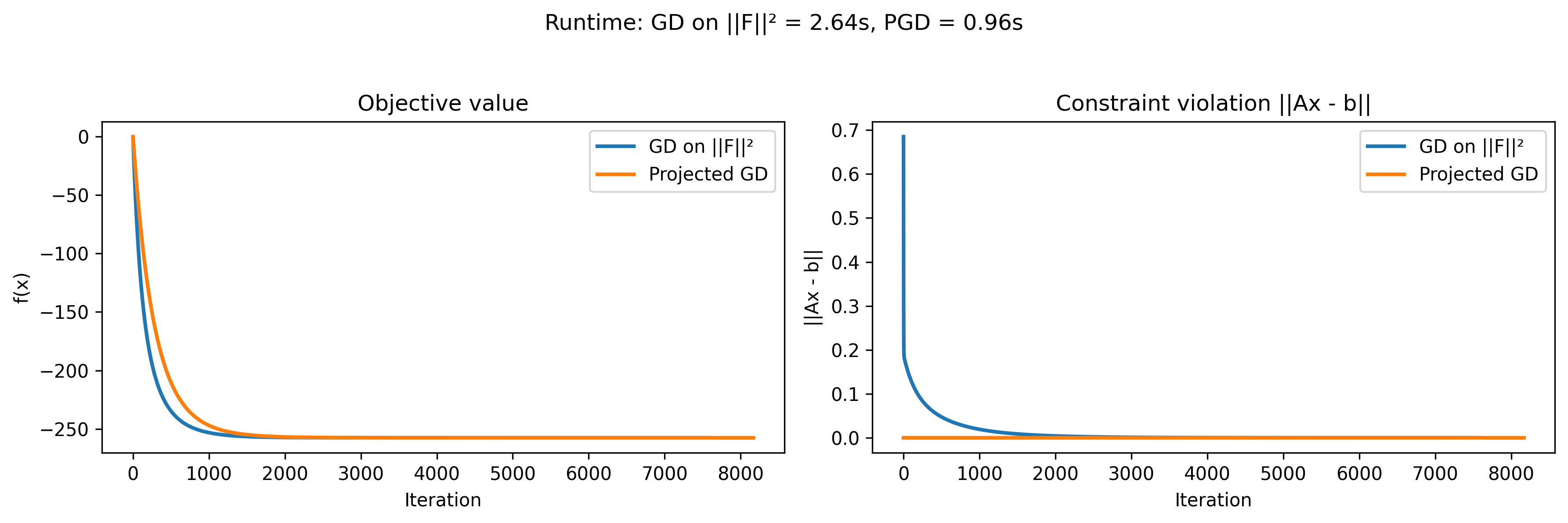
Just an example of minimizing the norm of the gradient (root seeking) of the lagrangian and Projected GD. The function under consideration is $\frac{1}{2}x^{\top}Qx + qx$. In this case $x \in R^{1000}$ and $A \in R^{100\times 1000}$. For both algorithms a fixed step size of 0.001 is (just to keep it simple), loop stops if gradient is below 0.0001.

Importantly, while projected gradient descent enforces feasibility during the whole training process, minimizing the norm of the gradient of the Lagrangian reaches feasibility asymptotically.

Newton’s method application

While gradient descent cannot be applied directly, Newton’s method is a root seeking algorithm so it might be applied directly to the Lagrangian⁶ . We can start from equations in \ref{eq:derivatives_const}, then calculate the second derivative and we have the Newton system:

\[\begin{pmatrix} \nabla^2 f(x_k) & A^\top \\ A & 0 \end{pmatrix} \begin{pmatrix} \Delta x_k \\ \Delta \nu_k \end{pmatrix} = -\begin{pmatrix} \nabla f(x_k) + A^\top \nu_k \\ Ax_k - b \end{pmatrix} = -\begin{pmatrix} \nabla f(x_k) + A^\top \nu_k \\ 0 \end{pmatrix}\]

and the update is

\[x_{k+1} = x_k - \Delta x_k, \quad \nu_{k+1} = \nu_k - \Delta \nu_k.\]

There is an important distinction in the actual algorithm if the start is or not feasible (\(Ax = b\)). If the start is not feasible we are essentially looking at a primal-dual optimization algorithm and we look at minimizing the residual vector. This has implications in the line search, convergence criteria and so on. The second equality in the Newton system would not be true in that case. However, it is often pretty simple to provide a feasible starting point. In that case, we can actually do some simple algebra

\[\begin{aligned} \nabla^2 f(x_k) \Delta x_k + A^\top \Delta \nu_k &= - \nabla f(x_k) - A^\top \nu_k \\ \nabla^2 f(x_k) \Delta x_k &= - \nabla f(x_k) - A^\top (\nu_k + \Delta \nu_k) \end{aligned}\]

so let \(\nu = (\nu_k + \Delta \nu_k)\) to reach the equivalent simpler system:

\[\begin{pmatrix} \nabla^2 f(x_k) & A^\top \\ A & 0 \end{pmatrix} \begin{pmatrix} \Delta x_k \\ \nu \end{pmatrix} = -\begin{pmatrix} \nabla f(x_k) \\ 0 \end{pmatrix}.\]

In the latter we actually do not care much about \(\nu\) until convergence. Since it does not play any role in determining the updates for \(x\).

In the above example, a very naive implementation of Newton’s method takes only 0.068 seconds.

---

References

These notes are a personal synthesis and extensions based on lectures from Mastermath (NL) Continuous Optimization Course 2025 along with standard references (below). Any errors are my own.

1. Boyd, S., & Vandenberghe, L.
   Convex Optimization

Footnotes

1. Why convexity requires second derivative PSD?

The first order condition for convexity: \[ f(y) \geq f(x) + \nabla f(x)^{\top}(y-x) \forall x, y: \]

Now, again making use of the Lagrange remainder is easy to see that the second derivative must be greater or equal to 0 in the scalar case or PSD in the vector case: \[ f(y) = f(x) + \nabla f(x)^{\top}(y-x) + \frac{1}{2} (y-x)^{\top}\nabla ^2 f(z) (y - x) \geq f(x) + \nabla f(x)^{\top}(y-x) \]

2. Why the smallest eigenvalue gives a lower bound?

Let the Hessian (which is always symmetric) at \(z\) have an eigendecomposition \[ \nabla^2 f(z) = Q \nu Q^{\top}, \] where \(Q\) is an orthogonal matrix of eigenvectors, and \(\nu = \mathrm{diag}(\nu_1, \ldots, \nu_n)\) contains the real eigenvalues. In this basis, write \(v = Q^{\top}(y-x)\). Then the quadratic form becomes \[ (y-x)^{\top}\nabla^2 f(z)(y-x) = v^{\top}\nu v = \sum_{i=1}^n \nu_i v_i^2. \] Since each \(v_i^2 \ge 0\), we have \[ \sum_{i=1}^n \nu_i v_i^2 \ge \nu_{\min} \sum_{i=1}^n v_i^2 = \nu_{\min} \|v\|^2_2 = \nu_{\min} \|y-x\|^2_2. \] Therefore, \[ \frac{1}{2}(y-x)^{\top}\nabla^2 f(z)(y-x) \ge \frac{1}{2}\nu_{\min}\,\|y-x\|^2_2. \]

3. Derivation using primal/dual arguments

This way is longer but for me seems more intuitive: We derive the primal solution analytically, this is indeed a minimizer if $\nu > 0$, since then, the Lagrangian is bounded below w.r.t $v$: \[ L(v, \nu) = \nabla f(x) + \nu \bigg(v^\top P v - 1\bigg). \] Differentiating and equating to 0 (very easy) we find that: \[ v = -P^{-1}\frac{\nabla f(x)}{2\nu}. \] Good, now plugging this in we got rid of $v$ and we focus on maximizing the dual function: \[ \begin{aligned} g(\nu) &= \min_v L(v, \nu) \\ &= \nabla f(x)^\top \Big(-\frac{1}{2\nu} P^{-1} \nabla f(x)\Big) + \nu \Big( \big(-\frac{1}{2\nu} P^{-1} \nabla f(x)\big)^\top P \big(-\frac{1}{2\nu} P^{-1} \nabla f(x)\big) - 1 \Big) \\ &= -\frac{1}{4\nu} \nabla f(x)^\top P^{-1} \nabla f(x) - \nu \end{aligned} \] Maximizing over \(\nu > 0\) gives \[ \frac{d g}{d \nu} = \frac{1}{4 \nu^2} \nabla f(x)^\top P^{-1} \nabla f(x) - 1 = 0 \quad \rightarrow \quad \nu = \frac{1}{2} \sqrt{\nabla f(x)^\top P^{-1} \nabla f(x)} \] Plugging \(\nu\) back into \(v(\nu)\) recovers the primal solution: \[ v = - \frac{P^{-1} \nabla f(x)}{\sqrt{\nabla f(x)^\top P^{-1} \nabla f(x)}} = \frac{P^{-1}\nabla f(x)}{\| P^{-0.5}\nabla f(x) \|_2}. \]

4. Some other derivations from here...

Hessian: \[ \nabla^2 \bar{f}(\bar{x}) = A^{-\top} \nabla^2 f(A^{-1}\bar{x}) A^{-1} = A^{-\top} \nabla^2 f(x) A^{-1} \] If we look at directional derivatives and quadratic form with the Hessian then we have: \[ \begin{aligned} \nabla \bar{f}(\bar{x})^{\top} \color{green}{v} &= \nabla \bar{f}(\bar{x})^{\top} \color{green}{v} \\ &= \nabla f(x)^{\top} \color{green}{A^{-1} v} \\ \end{aligned} \] and \[ \begin{aligned} \color{green}{v^{\top}} \color{white}{\nabla^2 \bar{f}(\bar{x}) } \color{green}{v} \color{white}{=} \color{green}{\bigg(A^{-1}v\bigg)^{\top}} \color{white}{\nabla^2 f(x) } \color{green}{\bigg(A^{-1}v\bigg)}. \end{aligned} \]

5. Proof for $f(x) - x^* \leq \frac{1}{2m} \| \nabla f(x)\|_2^2$

Start with second order Taylor expansion with Lagrange remainder and continue using the lower bound on the minimum eigenvalue of the Hessian: \[ \begin{aligned} f(y) &= f(x) + \nabla f(x)^{\top}(y-x) + \frac{1}{2}(y-x)\nabla ^2 f(z)(y-x) \\ &\geq f(x) + \nabla f(x)^{\top}(y-x) + \frac{1}{2}(y-x)\nabla ^2 mI(y-x) \\ &= f(x) + \nabla f(x)^{\top}(y-x) + \frac{m}{2}\|(y-x)\|_2^2 .\\ \end{aligned} \] Now, minimize with respect to $y$. This is clearly a lower bound. \[ \begin{aligned} f(y) &\geq \text{minimize}_w \nabla f(x)^{\top}(w-x) + \frac{m}{2}\|(w-x)\|_2^2\\ &= f(x) - \frac{1}{2m} \| \nabla f(x)\|^2_2. \end{aligned} \] Note the solution to the minimization problem: \[ \nabla f(x) + m(w + x) = 0 \rightarrow w = x - \frac{1}{m} \nabla f(x). \] Finally, $f(y)\geq f(x) - \frac{1}{2m} \| \nabla f(x)\|^2_2 \rightarrow f(x) - f(y) \leq \frac{1}{2m} \| \nabla f(x)\|^2_2$. Since this holds for any $y$ we can plug in the optimum value of the parameters and hence $f(x) - x^* \leq \frac{1}{2m} \| \nabla f(x)\|_2^2$.

6.

I am actually struggling to frame this under the condition number correction... So I will just give the traditional justifications.

---

<

Previous Post

Pendulum, equations of motion from first principles and solutions using ML.

>

Next Post

Inequality constrained optimization (SVM "the technical problem").